

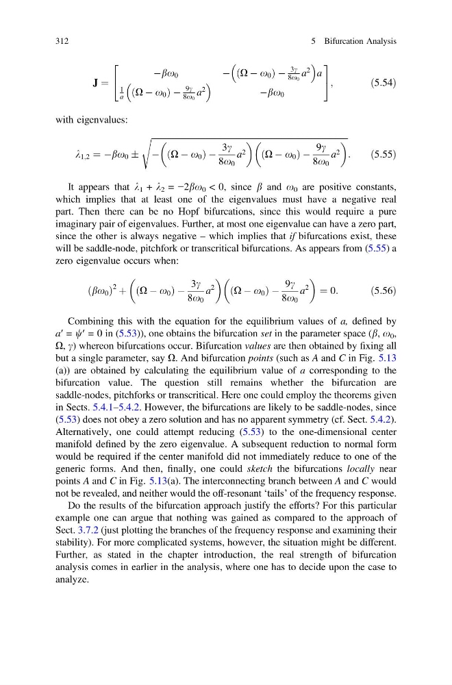
J ¼
Àbx 0
À ðX À x 0 Þ À
3c
8x 0
a
2
a
1
a ðX À x 0 Þ À
9c
8x 0
a
2
Àbx 0
2
4
3
5 ;
ð5:54Þ
with eigenvalues:
k 1;2 ¼ Àbx 0 Æ
ffiffiffiffiffiffiffiffiffiffiffiffiffiffiffiffiffiffiffiffiffiffiffiffiffiffiffiffiffiffiffiffiffiffiffiffiffiffiffiffiffiffiffiffiffiffiffiffiffiffiffiffiffiffiffiffiffiffiffiffiffiffiffiffiffiffiffiffiffiffiffiffiffiffiffiffiffiffiffiffiffiffiffiffiffiffiffiffiffiffiffiffi
À ðX À x 0 Þ À
3c
8x 0
a 2
ðX À x 0 Þ À
9c
8x 0
a 2
s
:
ð5:55Þ
It appears that k 1 + k 2 = −2bx 0 < 0, since b and x 0 are positive constants,
which implies that at least one of the eigenvalues must have a negative real
part. Then there can be no Hopf bifurcations, since this would require a pure
imaginary pair of eigenvalues. Further, at most one eigenvalue can have a zero part,
since the other is always negative – which implies that if bifurcations exist, these
will be saddle-node, pitchfork or transcritical bifurcations. As appears from (5.55) a
zero eigenvalue occurs when:
ðbx 0 Þ
2 þ ðX À x 0 Þ À
3c
8x 0
a
2
ðX À x 0 Þ À
9c
8x 0
a
2
¼ 0:
ð5:56Þ
Combining this with the equation for the equilibrium values of a, defined by
a′ = w′ = 0 in (5.53)), one obtains the bifurcation set in the parameter space (b, x 0 ,
X, c) whereon bifurcations occur. Bifurcation values are then obtained by fixing all
but a single parameter, say X. And bifurcation points (such as A and C in Fig. 5.13
(a)) are obtained by calculating the equilibrium value of a corresponding to the
bifurcation value. The question still remains whether the bifurcation are
saddle-nodes, pitchforks or transcritical. Here one could employ the theorems given
in Sects. 5.4.1–5.4.2. However, the bifurcations are likely to be saddle-nodes, since
(5.53) does not obey a zero solution and has no apparent symmetry (cf. Sect. 5.4.2).
Alternatively, one could attempt reducing (5.53) to the one-dimensional center
manifold defined by the zero eigenvalue. A subsequent reduction to normal form
would be required if the center manifold did not immediately reduce to one of the
generic forms. And then, finally, one could sketch the bifurcations locally near
points A and C in Fig. 5.13(a). The interconnecting branch between A and C would
not be revealed, and neither would the off-resonant ‘tails’ of the frequency response.
Do the results of the bifurcation approach justify the efforts? For this particular
example one can argue that nothing was gained as compared to the approach of
Sect. 3.7.2 (just plotting the branches of the frequency response and examining their
stability). For more complicated systems, however, the situation might be different.
Further, as stated in the chapter introduction, the real strength of bifurcation
analysis comes in earlier in the analysis, where one has to decide upon the case to
analyze.
312
5 Bifurcation Analysis
Àbx 0
À ðX À x 0 Þ À
3c
8x 0
a
2
a
1
a ðX À x 0 Þ À
9c
8x 0
a
2
Àbx 0
2
4
3
5 ;
ð5:54Þ
with eigenvalues:
k 1;2 ¼ Àbx 0 Æ
ffiffiffiffiffiffiffiffiffiffiffiffiffiffiffiffiffiffiffiffiffiffiffiffiffiffiffiffiffiffiffiffiffiffiffiffiffiffiffiffiffiffiffiffiffiffiffiffiffiffiffiffiffiffiffiffiffiffiffiffiffiffiffiffiffiffiffiffiffiffiffiffiffiffiffiffiffiffiffiffiffiffiffiffiffiffiffiffiffiffiffiffi
À ðX À x 0 Þ À
3c
8x 0
a 2
ðX À x 0 Þ À
9c
8x 0
a 2
s
:
ð5:55Þ
It appears that k 1 + k 2 = −2bx 0 < 0, since b and x 0 are positive constants,
which implies that at least one of the eigenvalues must have a negative real
part. Then there can be no Hopf bifurcations, since this would require a pure
imaginary pair of eigenvalues. Further, at most one eigenvalue can have a zero part,
since the other is always negative – which implies that if bifurcations exist, these
will be saddle-node, pitchfork or transcritical bifurcations. As appears from (5.55) a
zero eigenvalue occurs when:
ðbx 0 Þ
2 þ ðX À x 0 Þ À
3c
8x 0
a
2
ðX À x 0 Þ À
9c
8x 0
a
2
¼ 0:
ð5:56Þ
Combining this with the equation for the equilibrium values of a, defined by
a′ = w′ = 0 in (5.53)), one obtains the bifurcation set in the parameter space (b, x 0 ,
X, c) whereon bifurcations occur. Bifurcation values are then obtained by fixing all
but a single parameter, say X. And bifurcation points (such as A and C in Fig. 5.13
(a)) are obtained by calculating the equilibrium value of a corresponding to the
bifurcation value. The question still remains whether the bifurcation are
saddle-nodes, pitchforks or transcritical. Here one could employ the theorems given
in Sects. 5.4.1–5.4.2. However, the bifurcations are likely to be saddle-nodes, since
(5.53) does not obey a zero solution and has no apparent symmetry (cf. Sect. 5.4.2).
Alternatively, one could attempt reducing (5.53) to the one-dimensional center
manifold defined by the zero eigenvalue. A subsequent reduction to normal form
would be required if the center manifold did not immediately reduce to one of the
generic forms. And then, finally, one could sketch the bifurcations locally near
points A and C in Fig. 5.13(a). The interconnecting branch between A and C would
not be revealed, and neither would the off-resonant ‘tails’ of the frequency response.
Do the results of the bifurcation approach justify the efforts? For this particular
example one can argue that nothing was gained as compared to the approach of
Sect. 3.7.2 (just plotting the branches of the frequency response and examining their
stability). For more complicated systems, however, the situation might be different.
Further, as stated in the chapter introduction, the real strength of bifurcation
analysis comes in earlier in the analysis, where one has to decide upon the case to
analyze.
312
5 Bifurcation Analysis