both a and x functions of s, so that the solution curve is described by a set of points
(a(s), x(s)), with s belonging to some relevant interval.
To calculate the relation between changes in a and changes in x on the solution
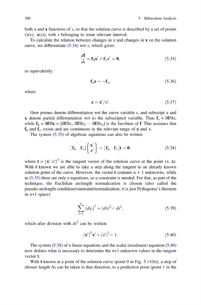
curve, we differentiate (5.34) wrt s, which gives:
df
ds
¼ f x x
0
þ f a a
0
¼ 0;
ð5:35Þ
or equivalently:
f x z ¼ Àf a ;
ð5:36Þ
where
z ¼ x
0
=a
0
:
ð5:37Þ
Here primes denote differentiation wrt the curve variable s, and subscript a and
x denote partial differentiation wrt to the subscripted variable. Thus f a = ∂f/∂a,
while f x = ∂f/∂x = [∂f/∂x 1 ∂f/∂x 2 ÁÁÁ ∂f/∂x n ] is the Jacobian of f. This assumes that
f x and f a . exists and are continuous in the relevant range of x and a.
The system (5.35) of algebraic equations can also be written
f x f a
½
Š
x
0
a
0
& '
¼ f x f a
½
Št ¼ 0;
ð5:38Þ
where t = {x′ a′}
T is the tangent vector of the solution curve at the point (a, x).
With t known we are able to take a step along the tangent to an already known
solution point of the curve. However, the vector t contains n + 1 unknowns, while
in (5.35) there are only n equations, so a constraint is needed. For that, as part of the
technique, the Euclidian arclength normalization is chosen (also called the
pseudo-arclength condition/constraint/normalization; it is just Pythagoras’s theorem
in n+1 space):
X n
j¼1
dx j
À Á 2 þ da
ð Þ
2 ¼ ds
2
;
ð5:39Þ
which after division with ds
2 can be written:
x
0
ð Þ
T x
0
þ a
0
ð Þ
2 ¼ 1:
ð5:40Þ
The system (5.38) of n linear equations and the scalar (nonlinear) equation (5.40)
now defines what is necessary to determine the n+1 unknown values in the tangent
vector t.
With t known at a point of the solution curve (point 0 in Fig. 5.11(b)), a step of
chosen length Ds can be taken in that direction, to a prediction point (point 1 in the
300
5 Bifurcation Analysis