

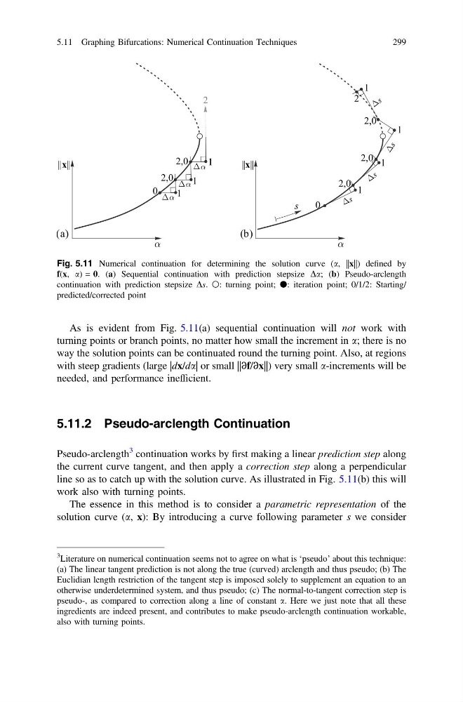
As is evident from Fig. 5.11(a) sequential continuation will not work with
turning points or branch points, no matter how small the increment in a; there is no
way the solution points can be continuated round the turning point. Also, at regions
with steep gradients (large |dx/da| or small ||∂f/∂x||) very small a-increments will be
needed, and performance inefficient.
5.11.2 Pseudo-arclength Continuation
Pseudo-arclength
3 continuation works by first making a linear prediction step along
the current curve tangent, and then apply a correction step along a perpendicular
line so as to catch up with the solution curve. As illustrated in Fig. 5.11(b) this will
work also with turning points.
The essence in this method is to consider a parametric representation of the
solution curve (a, x): By introducing a curve following parameter s we consider
Fig. 5.11 Numerical continuation for determining the solution curve (a, ||x||) defined by
f(x, a) = 0. (a) Sequential continuation with prediction stepsize Da; (b) Pseudo-arclength
continuation with prediction stepsize Ds. ○: turning point; ●: iteration point; 0/1/2: Starting/
predicted/corrected point
3
Literature on numerical continuation seems not to agree on what is ‘pseudo’ about this technique:
(a) The linear tangent prediction is not along the true (curved) arclength and thus pseudo; (b) The
Euclidian length restriction of the tangent step is imposed solely to supplement an equation to an
otherwise underdetermined system, and thus pseudo; (c) The normal-to-tangent correction step is
pseudo-, as compared to correction along a line of constant a. Here we just note that all these
ingredients are indeed present, and contributes to make pseudo-arclength continuation workable,
also with turning points.
5.11 Graphing Bifurcations: Numerical Continuation Techniques
299
turning points or branch points, no matter how small the increment in a; there is no
way the solution points can be continuated round the turning point. Also, at regions
with steep gradients (large |dx/da| or small ||∂f/∂x||) very small a-increments will be
needed, and performance inefficient.
5.11.2 Pseudo-arclength Continuation
Pseudo-arclength
3 continuation works by first making a linear prediction step along
the current curve tangent, and then apply a correction step along a perpendicular
line so as to catch up with the solution curve. As illustrated in Fig. 5.11(b) this will
work also with turning points.
The essence in this method is to consider a parametric representation of the
solution curve (a, x): By introducing a curve following parameter s we consider
Fig. 5.11 Numerical continuation for determining the solution curve (a, ||x||) defined by
f(x, a) = 0. (a) Sequential continuation with prediction stepsize Da; (b) Pseudo-arclength
continuation with prediction stepsize Ds. ○: turning point; ●: iteration point; 0/1/2: Starting/
predicted/corrected point
3
Literature on numerical continuation seems not to agree on what is ‘pseudo’ about this technique:
(a) The linear tangent prediction is not along the true (curved) arclength and thus pseudo; (b) The
Euclidian length restriction of the tangent step is imposed solely to supplement an equation to an
otherwise underdetermined system, and thus pseudo; (c) The normal-to-tangent correction step is
pseudo-, as compared to correction along a line of constant a. Here we just note that all these
ingredients are indeed present, and contributes to make pseudo-arclength continuation workable,
also with turning points.
5.11 Graphing Bifurcations: Numerical Continuation Techniques
299