

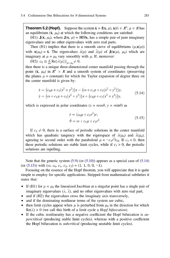
Theorem 5.2 (Hopf). Suppose the system _
x = f(x, l), x(t) 2 R
n , l 2 R has
an equilibrium (~ x, l 0 ) at which the following conditions are satisfied:
(H1): J(~ x, l 0 ), where J(x, l) = ∂f/∂x, has a simple pair of pure imaginary
eigenvalues and no other eigenvalues with zero real parts.
Then (H1) implies that there is a smooth curve of equilibriums (l,x(l))
with x(l 0 ) = ~ x. The eigenvalues k(l) and k(l) of J(x(l), l 0 ) which are
imaginary at l = l 0 vary smoothly with l. If, moreover:
(H2): c 0
d
dl Re kðlÞ
ð
Þj l¼l 0 6 ¼ 0;
then there is a unique three-dimensional center manifold passing through the
point (~ x, l 0 ) in R
n
 R and a smooth system of coordinates (preserving
the planes l = constant) for which the Taylor expansion of degree three on
the center manifold is given by:
_
x ¼ c 0 l þ c 3 ðx
2
þ y
2
Þ
À
Á
x À x þ c 1 l þ c 2 ðx
2
þ y
2
Þ
À
Á
y;
_
y ¼ x þ c 1 l þ c 2 ðx
2
þ y
2
Þ
À
Á
x þ c 0 l þ c 3 ðx
2
þ y
2
Þ
À
Á
y;
ð5:14Þ
which is expressed in polar coordinates (x = rcosh, y = rsinh) as
_
r ¼ ðc 0 l þ c 3 r
2
Þr;
_
h ¼ x þ c 1 l þ c 2 r
2
:
ð5:15Þ
If c 3 6 ¼ 0, there is a surface of periodic solutions in the center manifold
which has quadratic tangency with the eigenspace of k(l 0 ) and k(l 0 ),
agreeing to second order with the paraboloid l = −c 3 r
2 /c 0 . If c 3 < 0, then
these periodic solutions are stable limit cycles, while if c 3 > 0, the periodic
solutions are repelling.
Note that the generic system (5.9) (or (5.10)) appears as a special case of (5.14)
(or (5.15)) with (x, c 0 , c 1 , c 2 , c 3 ) = (1, 1, 0, 0, −1).
Focusing on the essence of the Hopf theorem, you will appreciate that it is quite
simple to employ for specific applications. Stripped from mathematical subtleties it
states that:
• If (H1) for l = l 0 the linearized Jacobian at a singular point has a single pair of
imaginary eigenvalues (k, k), and no other eigenvalues with zero real part,
• and if (H2) the eigenvalues cross the imaginary axis transversely,
• and if the dominating nonlinear terms of the system are cubic,
• then limit cycles appear when l is perturbed from l 0 in the direction for which
Re(k) > 0 (we call this birth of a limit cycle a Hopf bifurcation).
• If the cubic nonlinearity has a negative coefficient the Hopf bifurcation is supercritical (producing stable limit cycles), whereas with a positive coefficient
the Hopf bifurcation is subcritical (producing unstable limit cycles).
5.4 Codimension One Bifurcations for N-dimensional Systems
283
x = f(x, l), x(t) 2 R
n , l 2 R has
an equilibrium (~ x, l 0 ) at which the following conditions are satisfied:
(H1): J(~ x, l 0 ), where J(x, l) = ∂f/∂x, has a simple pair of pure imaginary
eigenvalues and no other eigenvalues with zero real parts.
Then (H1) implies that there is a smooth curve of equilibriums (l,x(l))
with x(l 0 ) = ~ x. The eigenvalues k(l) and k(l) of J(x(l), l 0 ) which are
imaginary at l = l 0 vary smoothly with l. If, moreover:
(H2): c 0
d
dl Re kðlÞ
ð
Þj l¼l 0 6 ¼ 0;
then there is a unique three-dimensional center manifold passing through the
point (~ x, l 0 ) in R
n
 R and a smooth system of coordinates (preserving
the planes l = constant) for which the Taylor expansion of degree three on
the center manifold is given by:
_
x ¼ c 0 l þ c 3 ðx
2
þ y
2
Þ
À
Á
x À x þ c 1 l þ c 2 ðx
2
þ y
2
Þ
À
Á
y;
_
y ¼ x þ c 1 l þ c 2 ðx
2
þ y
2
Þ
À
Á
x þ c 0 l þ c 3 ðx
2
þ y
2
Þ
À
Á
y;
ð5:14Þ
which is expressed in polar coordinates (x = rcosh, y = rsinh) as
_
r ¼ ðc 0 l þ c 3 r
2
Þr;
_
h ¼ x þ c 1 l þ c 2 r
2
:
ð5:15Þ
If c 3 6 ¼ 0, there is a surface of periodic solutions in the center manifold
which has quadratic tangency with the eigenspace of k(l 0 ) and k(l 0 ),
agreeing to second order with the paraboloid l = −c 3 r
2 /c 0 . If c 3 < 0, then
these periodic solutions are stable limit cycles, while if c 3 > 0, the periodic
solutions are repelling.
Note that the generic system (5.9) (or (5.10)) appears as a special case of (5.14)
(or (5.15)) with (x, c 0 , c 1 , c 2 , c 3 ) = (1, 1, 0, 0, −1).
Focusing on the essence of the Hopf theorem, you will appreciate that it is quite
simple to employ for specific applications. Stripped from mathematical subtleties it
states that:
• If (H1) for l = l 0 the linearized Jacobian at a singular point has a single pair of
imaginary eigenvalues (k, k), and no other eigenvalues with zero real part,
• and if (H2) the eigenvalues cross the imaginary axis transversely,
• and if the dominating nonlinear terms of the system are cubic,
• then limit cycles appear when l is perturbed from l 0 in the direction for which
Re(k) > 0 (we call this birth of a limit cycle a Hopf bifurcation).
• If the cubic nonlinearity has a negative coefficient the Hopf bifurcation is supercritical (producing stable limit cycles), whereas with a positive coefficient
the Hopf bifurcation is subcritical (producing unstable limit cycles).
5.4 Codimension One Bifurcations for N-dimensional Systems
283