

5.4.1 Saddle-Node Conditions
Here are the necessary conditions for saddle-node bifurcations to occur (adopted
from Guckenheimer and Holmes 1983):
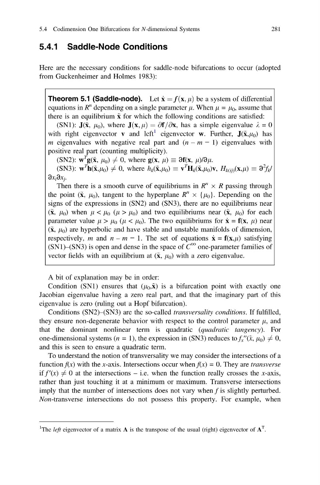
Theorem 5.1 (Saddle-node). Let _
x ¼ f ðx; lÞ be a system of differential
equations in R
n depending on a single parameter l. When l = l 0 , assume that
there is an equilibrium ~ x for which the following conditions are satisfied:
(SN1): J(~ x, l 0 ), where Jðx; lÞ ¼ @f=@x, has a simple eigenvalue k = 0
with right eigenvector v and left
1 eigenvector w. Further, J(~ x,l 0 ) has
m eigenvalues with negative real part and (n – m − 1) eigenvalues with
positive real part (counting multiplicity).
(SN2): w
T
g(~ x, l 0 ) 6 ¼ 0, where g(x, l) ∂f(x, l)/∂l.
(SN3): w
T
h(~ x,l 0 ) 6 ¼ 0, where h k (~ x,l 0 ) v
T
H k (~ x,l 0 )v, H k(ij) (x,l) ∂
2 f k /
∂x i ∂x j .
Then there is a smooth curve of equilibriums in R
n
 R passing through
the point (~ x, l 0 ), tangent to the hyperplane R
n
 {l 0 }. Depending on the
signs of the expressions in (SN2) and (SN3), there are no equilibriums near
(~ x, l 0 ) when l < l 0 (l > l 0 ) and two equilibriums near (~ x, l 0 ) for each
parameter value l > l 0 (l < l 0 ). The two equilibriums for _
x = f(x, l) near
(~ x, l 0 ) are hyperbolic and have stable and unstable manifolds of dimension,
respectively, m and n – m − 1. The set of equations _
x = f(x,l) satisfying
(SN1)–(SN3) is open and dense in the space of C
∞ one-parameter families of
vector fields with an equilibrium at (~ x, l 0 ) with a zero eigenvalue.
A bit of explanation may be in order:
Condition (SN1) ensures that (l 0 ,~ x) is a bifurcation point with exactly one
Jacobian eigenvalue having a zero real part, and that the imaginary part of this
eigenvalue is zero (ruling out a Hopf bifurcation).
Conditions (SN2)–(SN3) are the so-called transversality conditions. If fulfilled,
they ensure non-degenerate behavior with respect to the control parameter l, and
that the dominant nonlinear term is quadratic (quadratic tangency). For
one-dimensional systems (n = 1), the expression in (SN3) reduces to f x ′′(~ x, l 0 ) 6 ¼ 0,
and this is seen to ensure a quadratic term.
To understand the notion of transversality we may consider the intersections of a
function f(x) with the x-axis. Intersections occur when f(x) = 0. They are transverse
if f ′(x) 6 ¼ 0 at the intersections – i.e. when the function really crosses the x-axis,
rather than just touching it at a minimum or maximum. Transverse intersections
imply that the number of intersections does not vary when f is slightly perturbed.
Non-transverse intersections do not possess this property. For example, when
1
The left eigenvector of a matrix A is the transpose of the usual (right) eigenvector of A
T .
5.4 Codimension One Bifurcations for N-dimensional Systems
281
Here are the necessary conditions for saddle-node bifurcations to occur (adopted
from Guckenheimer and Holmes 1983):
Theorem 5.1 (Saddle-node). Let _
x ¼ f ðx; lÞ be a system of differential
equations in R
n depending on a single parameter l. When l = l 0 , assume that
there is an equilibrium ~ x for which the following conditions are satisfied:
(SN1): J(~ x, l 0 ), where Jðx; lÞ ¼ @f=@x, has a simple eigenvalue k = 0
with right eigenvector v and left
1 eigenvector w. Further, J(~ x,l 0 ) has
m eigenvalues with negative real part and (n – m − 1) eigenvalues with
positive real part (counting multiplicity).
(SN2): w
T
g(~ x, l 0 ) 6 ¼ 0, where g(x, l) ∂f(x, l)/∂l.
(SN3): w
T
h(~ x,l 0 ) 6 ¼ 0, where h k (~ x,l 0 ) v
T
H k (~ x,l 0 )v, H k(ij) (x,l) ∂
2 f k /
∂x i ∂x j .
Then there is a smooth curve of equilibriums in R
n
 R passing through
the point (~ x, l 0 ), tangent to the hyperplane R
n
 {l 0 }. Depending on the
signs of the expressions in (SN2) and (SN3), there are no equilibriums near
(~ x, l 0 ) when l < l 0 (l > l 0 ) and two equilibriums near (~ x, l 0 ) for each
parameter value l > l 0 (l < l 0 ). The two equilibriums for _
x = f(x, l) near
(~ x, l 0 ) are hyperbolic and have stable and unstable manifolds of dimension,
respectively, m and n – m − 1. The set of equations _
x = f(x,l) satisfying
(SN1)–(SN3) is open and dense in the space of C
∞ one-parameter families of
vector fields with an equilibrium at (~ x, l 0 ) with a zero eigenvalue.
A bit of explanation may be in order:
Condition (SN1) ensures that (l 0 ,~ x) is a bifurcation point with exactly one
Jacobian eigenvalue having a zero real part, and that the imaginary part of this
eigenvalue is zero (ruling out a Hopf bifurcation).
Conditions (SN2)–(SN3) are the so-called transversality conditions. If fulfilled,
they ensure non-degenerate behavior with respect to the control parameter l, and
that the dominant nonlinear term is quadratic (quadratic tangency). For
one-dimensional systems (n = 1), the expression in (SN3) reduces to f x ′′(~ x, l 0 ) 6 ¼ 0,
and this is seen to ensure a quadratic term.
To understand the notion of transversality we may consider the intersections of a
function f(x) with the x-axis. Intersections occur when f(x) = 0. They are transverse
if f ′(x) 6 ¼ 0 at the intersections – i.e. when the function really crosses the x-axis,
rather than just touching it at a minimum or maximum. Transverse intersections
imply that the number of intersections does not vary when f is slightly perturbed.
Non-transverse intersections do not possess this property. For example, when
1
The left eigenvector of a matrix A is the transpose of the usual (right) eigenvector of A
T .
5.4 Codimension One Bifurcations for N-dimensional Systems
281