

Problem 4.11 Test engineers A and B have measured frequency response
functions as shown in Fig. P4.11 for transverse vibrations of a beam stiffener which
is critical to the safety of a larger structure. Fig. (a) shows the setup, and fig. (b) a
typical time series when the input is applied at beam point #11 and the acceleration
output is measured at point #2. Fig. (c) shows the corresponding frequency
response function (FRF), measured with the beam hung in two rubber bands.
Their next task is to make a mathematical model of the vibrating beam, and their
team manager wants a model that is as simple as possible. Test engineer A, to
whom this seems straightforward, suggests using the well-known linear partial
differential equation of motion describing flexural vibrations of a free-free uniform
beam. But to engineer B the situation appears more complicated: Having just
completed a course in advanced vibrations and stability, worries arise about
overlooking several intricate phenomena (which A is happily unaware about). In
particular, B wants to include the supporting rubber bands in the model, and to
include material nonlinearities and geometrical nonlinearities.
So: Is A’s suggestion for a model adequate for reproducing the most important
features of the experimental FRF in Figure (c)?
Useful information
• Beam data: Length l = 1 m, cross-section b  h = 40  10 mm, mass
M = 3120 grams, Young’s modulus E = 2.06 Â 10
11 Pa.
• The FRF measurements are in the form of accelerance, i.e. a(x)/f(x),
where a(x) and f(x), respectively, is the Fourier transform of the measured acceleration a(t) and force f(t).
• The six smallest solutions of cos(a) cosh(a) = 1 is: 4.730, 7.853, 11.00,
14.13, 17.28, 20.42.].
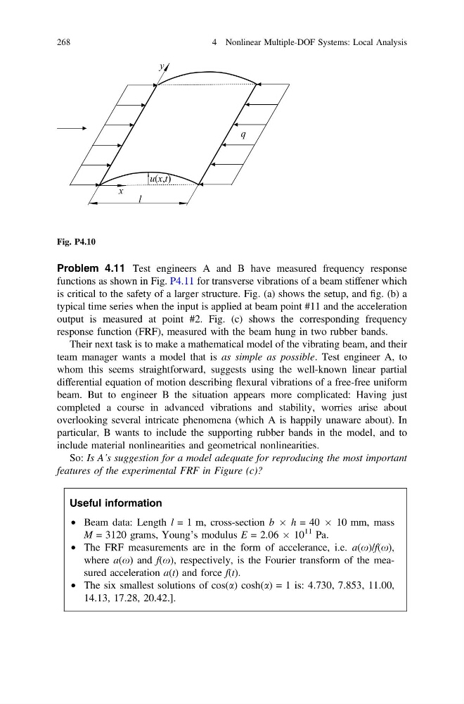
Fig. P4.10
268
4 Nonlinear Multiple-DOF Systems: Local Analysis
functions as shown in Fig. P4.11 for transverse vibrations of a beam stiffener which
is critical to the safety of a larger structure. Fig. (a) shows the setup, and fig. (b) a
typical time series when the input is applied at beam point #11 and the acceleration
output is measured at point #2. Fig. (c) shows the corresponding frequency
response function (FRF), measured with the beam hung in two rubber bands.
Their next task is to make a mathematical model of the vibrating beam, and their
team manager wants a model that is as simple as possible. Test engineer A, to
whom this seems straightforward, suggests using the well-known linear partial
differential equation of motion describing flexural vibrations of a free-free uniform
beam. But to engineer B the situation appears more complicated: Having just
completed a course in advanced vibrations and stability, worries arise about
overlooking several intricate phenomena (which A is happily unaware about). In
particular, B wants to include the supporting rubber bands in the model, and to
include material nonlinearities and geometrical nonlinearities.
So: Is A’s suggestion for a model adequate for reproducing the most important
features of the experimental FRF in Figure (c)?
Useful information
• Beam data: Length l = 1 m, cross-section b  h = 40  10 mm, mass
M = 3120 grams, Young’s modulus E = 2.06 Â 10
11 Pa.
• The FRF measurements are in the form of accelerance, i.e. a(x)/f(x),
where a(x) and f(x), respectively, is the Fourier transform of the measured acceleration a(t) and force f(t).
• The six smallest solutions of cos(a) cosh(a) = 1 is: 4.730, 7.853, 11.00,
14.13, 17.28, 20.42.].
Fig. P4.10
268
4 Nonlinear Multiple-DOF Systems: Local Analysis