

only for constant values of excitation frequency; they predict the stationary
amplitudes obtained after initial transients (the homogeneous part of the solution)
have decayed. They still remain valid if the frequency of excitation is changed very
slowly. When this is not the case, such as with experimental frequency-sweeps or
system startup/shutdowns at finite speed, the system will not have time to attain
stationary amplitudes. One then needs to consider transient response during the
passage of resonance. We thus reconsider the system (4.94) subjected to harmonic
base excitation w 0 (s) = w A sin(U(s)) at a slowly varying frequency. The amplitude
w A is constant, whereas U(s) = s + m(es), e ( 1, so that m is a slowly varying
function of time. The instantaneous frequency of excitation becomes X(s) =
= 1 + e _
m(es), and we then consider a passage through the region of primary
resonance X % 1 for the following system:
1 þ 2a sin
2
ðpyÞ
À
Á € u þ c 1 þ 2pa_ y sinð2pyÞ
ð
Þ _
u þ u
¼ w A
4
p
þ 2a sinðpyÞ
X
2 sin U À _
X cos U
À
Á ;
UðsÞ ¼
Z
XðsÞds;
€ y þ c 2 _
y þ f r ðyÞ ¼ À
1
2
p sinð2pyÞ€ uu:
ð4:104Þ
Methods for analyzing linear or nonlinear systems subjected to slowly varying
excitations are described in, e.g., Nayfeh and Mook (1979) and Evan-Iwanowski
(1976). For the present case we employ averaging.
With averaging the _
X-term in the first of Eq. (4.104) may be neglected when
compared to X
2 , since _
X = €
U = e
2
€ m ( X
2
% 1. A Van der Pol transformation (u, _
u)
! (a sinw, aX(s) cosw), where a = a(s) and w(s) = U(s) + h(s), is then applied to
0
0.16
0.6
0.8
1
1.2
1.4
String amplitude
a
Excitation frequency Ω
mass sliding
(a)
0.1
0.4
0.6
0.8
1
1.2
1.4
Pointmass position
y
Excitation frequency Ω
(b)
mass fixed
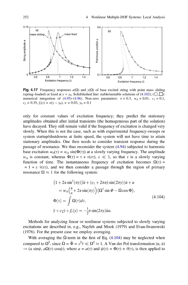
Fig. 4.17 Frequency responses a(X) and y(X) of base excited string with point mass sliding
(spring–loaded) or fixed at y = y 0 . Solid/dashed line: stable/unstable solutions of (4.102); ( ⃝, ⃞):
numerical integration of (4.95)–(4.96). Non-zero parameters: a = 0.3, w A = 0.01, c 1 = 0.1,
c 2 = 0.35, f r (y) = j(y – y 0 ), j = 0.03, y 0 = 0.1
252
4 Nonlinear Multiple-DOF Systems: Local Analysis
amplitudes obtained after initial transients (the homogeneous part of the solution)
have decayed. They still remain valid if the frequency of excitation is changed very
slowly. When this is not the case, such as with experimental frequency-sweeps or
system startup/shutdowns at finite speed, the system will not have time to attain
stationary amplitudes. One then needs to consider transient response during the
passage of resonance. We thus reconsider the system (4.94) subjected to harmonic
base excitation w 0 (s) = w A sin(U(s)) at a slowly varying frequency. The amplitude
w A is constant, whereas U(s) = s + m(es), e ( 1, so that m is a slowly varying
function of time. The instantaneous frequency of excitation becomes X(s) =
= 1 + e _
m(es), and we then consider a passage through the region of primary
resonance X % 1 for the following system:
1 þ 2a sin
2
ðpyÞ
À
Á € u þ c 1 þ 2pa_ y sinð2pyÞ
ð
Þ _
u þ u
¼ w A
4
p
þ 2a sinðpyÞ
X
2 sin U À _
X cos U
À
Á ;
UðsÞ ¼
Z
XðsÞds;
€ y þ c 2 _
y þ f r ðyÞ ¼ À
1
2
p sinð2pyÞ€ uu:
ð4:104Þ
Methods for analyzing linear or nonlinear systems subjected to slowly varying
excitations are described in, e.g., Nayfeh and Mook (1979) and Evan-Iwanowski
(1976). For the present case we employ averaging.
With averaging the _
X-term in the first of Eq. (4.104) may be neglected when
compared to X
2 , since _
X = €
U = e
2
€ m ( X
2
% 1. A Van der Pol transformation (u, _
u)
! (a sinw, aX(s) cosw), where a = a(s) and w(s) = U(s) + h(s), is then applied to
0
0.16
0.6
0.8
1
1.2
1.4
String amplitude
a
Excitation frequency Ω
mass sliding
(a)
0.1
0.4
0.6
0.8
1
1.2
1.4
Pointmass position
y
Excitation frequency Ω
(b)
mass fixed
Fig. 4.17 Frequency responses a(X) and y(X) of base excited string with point mass sliding
(spring–loaded) or fixed at y = y 0 . Solid/dashed line: stable/unstable solutions of (4.102); ( ⃝, ⃞):
numerical integration of (4.95)–(4.96). Non-zero parameters: a = 0.3, w A = 0.01, c 1 = 0.1,
c 2 = 0.35, f r (y) = j(y – y 0 ), j = 0.03, y 0 = 0.1
252
4 Nonlinear Multiple-DOF Systems: Local Analysis