

Fig. 4.3 shows the consequence of slight external detuning, r 1 = 0.2; That is, the
primary mass is not driven exactly at resonance X = x 1 . As appears, the absorber
still limits the a-response, though at a somewhat higher level. Comparing to the
case of perfect tuning the most noticeable difference is that jumps in the stationary
response now appear: Upon increasing the load-level q from below q 1 , the stationary absorber amplitude b raises abruptly from zero at q = q 2 . Similarly, upon
decreasing q from above q 2 there is a down-jump to zero at q = q 1 .
Fig. 4.5 is a frequency response, showing the vibration amplitude a of the
primary mass as a function of excitation frequency X, for three levels of loading
magnitude q. Note how the high amplitude linear resonance peaks near X = x 1 are
destabilized in the presence of nonlinear interaction. Effectively the peaks are ‘cut
off’, and the linear resonance at x 1 turns into a nonlinear anti-resonance.
Fig. 4.4 depicts the influence of slight internal detuning, that is, r 2 = x 1 –2x 2
differs slightly from zero so that the system is slightly offset from perfect internal
resonance. The frequency responses still limit the amplitude a of the primary mass,
albeit less efficiently than for perfect internal tuning, r 2 = 0.
4.2.4 Concluding Remarks on the Vibration
Absorber
Some of the nonlinear phenomena encountered in this section appear with
single-DOF systems as well. This concerns frequency locking, amplitude jumps and
the presence of multiple solution branches. Others are particular to multiple-DOF
systems: modal interaction, internal resonance and mode saturation. None of them
appear with linear systems. Hence, for the system considered – and others whose
mathematical model are similar to it – experimental observations cannot be
meaningfully explained by considering only the linearized equations of motion.
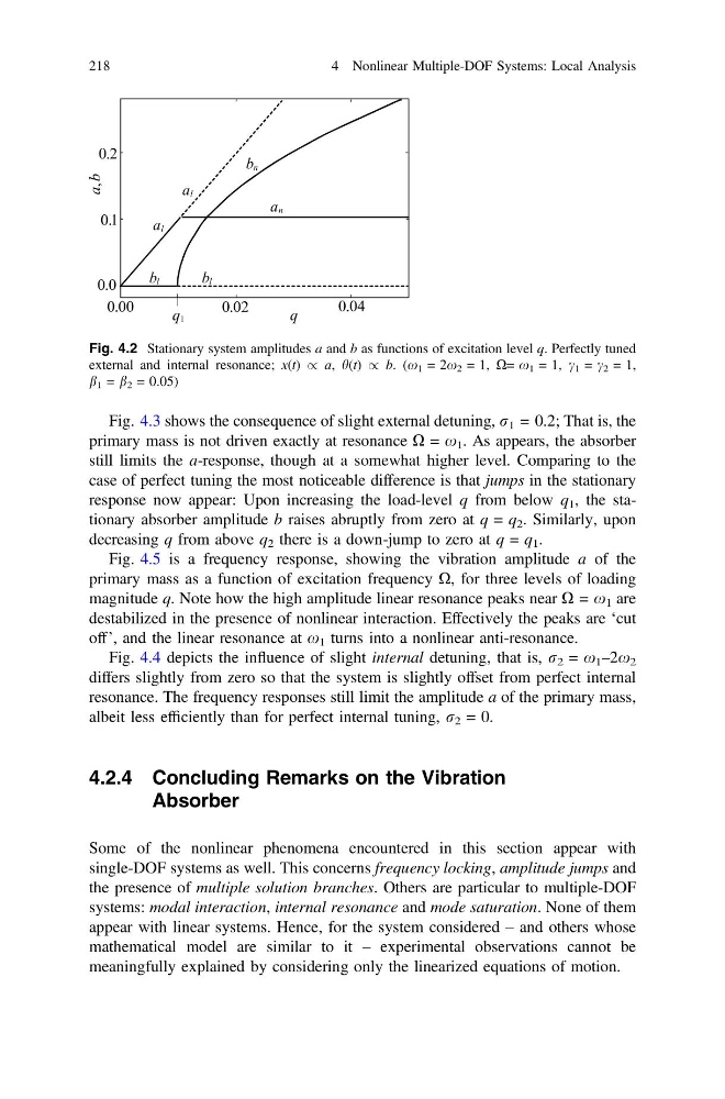
Fig. 4.2 Stationary system amplitudes a and b as functions of excitation level q. Perfectly tuned
external and internal resonance; x(t) / a, h(t) / b. (x 1 = 2x 2 = 1, X= x 1 = 1, c 1 = c 2 = 1,
b 1 = b 2 = 0.05)
218
4 Nonlinear Multiple-DOF Systems: Local Analysis
primary mass is not driven exactly at resonance X = x 1 . As appears, the absorber
still limits the a-response, though at a somewhat higher level. Comparing to the
case of perfect tuning the most noticeable difference is that jumps in the stationary
response now appear: Upon increasing the load-level q from below q 1 , the stationary absorber amplitude b raises abruptly from zero at q = q 2 . Similarly, upon
decreasing q from above q 2 there is a down-jump to zero at q = q 1 .
Fig. 4.5 is a frequency response, showing the vibration amplitude a of the
primary mass as a function of excitation frequency X, for three levels of loading
magnitude q. Note how the high amplitude linear resonance peaks near X = x 1 are
destabilized in the presence of nonlinear interaction. Effectively the peaks are ‘cut
off’, and the linear resonance at x 1 turns into a nonlinear anti-resonance.
Fig. 4.4 depicts the influence of slight internal detuning, that is, r 2 = x 1 –2x 2
differs slightly from zero so that the system is slightly offset from perfect internal
resonance. The frequency responses still limit the amplitude a of the primary mass,
albeit less efficiently than for perfect internal tuning, r 2 = 0.
4.2.4 Concluding Remarks on the Vibration
Absorber
Some of the nonlinear phenomena encountered in this section appear with
single-DOF systems as well. This concerns frequency locking, amplitude jumps and
the presence of multiple solution branches. Others are particular to multiple-DOF
systems: modal interaction, internal resonance and mode saturation. None of them
appear with linear systems. Hence, for the system considered – and others whose
mathematical model are similar to it – experimental observations cannot be
meaningfully explained by considering only the linearized equations of motion.
Fig. 4.2 Stationary system amplitudes a and b as functions of excitation level q. Perfectly tuned
external and internal resonance; x(t) / a, h(t) / b. (x 1 = 2x 2 = 1, X= x 1 = 1, c 1 = c 2 = 1,
b 1 = b 2 = 0.05)
218
4 Nonlinear Multiple-DOF Systems: Local Analysis