

€ x þ 2b_ x þ x
2 x ¼ 0 for x\D;
_
x þ ¼ À_ x À
for x ¼ D;
ð3:347Þ
where x ¼
ffiffiffiffiffiffiffiffi ffi
k=m
p
is the natural frequency of the unimpacting oscillator,
b ¼ c=ð2
ffiffiffiffiffiffi
km
p Þ is the viscous damping ratio, and the initial conditions are
xð0Þ ¼ x 0 ; _
xð0Þ ¼ v 0 :
a) Use a discontinuous transformation of variables, x = D – |z|, z + z – < 0, to
transform the equation of motion into a system with a discontinuity which is
small when x
2
D is small.
b) For the case D = 0, solve the transformed system for z(t), and use this to
calculate the exact solution for x(t) when x 0 = 0 and v 0 < 0.
c) Compute and graph the exact solution when b = 0.1, x = 1, D = 0, and
(x 0 , v 0 ) = (0, –0.1). Compare to results of numerical simulation, using e.g.
MATLAB and event-handling to solve the ODE numerically (here “an event” is
an impact, i.e. the condition x = D and _
x [ 0.
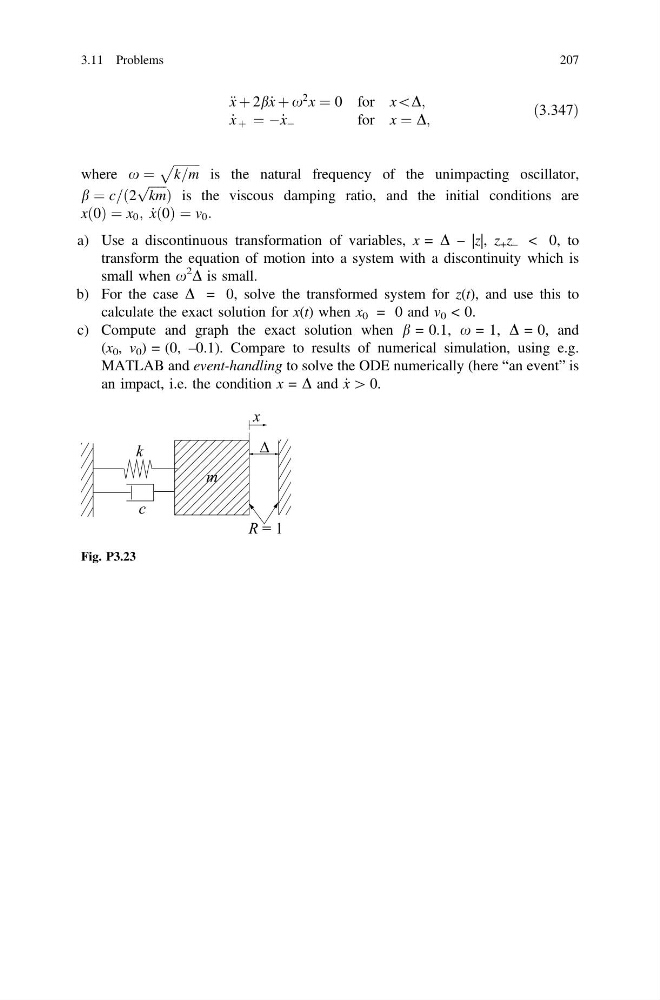
Fig. P3.23
3.11 Problems
207
2 x ¼ 0 for x\D;
_
x þ ¼ À_ x À
for x ¼ D;
ð3:347Þ
where x ¼
ffiffiffiffiffiffiffiffi ffi
k=m
p
is the natural frequency of the unimpacting oscillator,
b ¼ c=ð2
ffiffiffiffiffiffi
km
p Þ is the viscous damping ratio, and the initial conditions are
xð0Þ ¼ x 0 ; _
xð0Þ ¼ v 0 :
a) Use a discontinuous transformation of variables, x = D – |z|, z + z – < 0, to
transform the equation of motion into a system with a discontinuity which is
small when x
2
D is small.
b) For the case D = 0, solve the transformed system for z(t), and use this to
calculate the exact solution for x(t) when x 0 = 0 and v 0 < 0.
c) Compute and graph the exact solution when b = 0.1, x = 1, D = 0, and
(x 0 , v 0 ) = (0, –0.1). Compare to results of numerical simulation, using e.g.
MATLAB and event-handling to solve the ODE numerically (here “an event” is
an impact, i.e. the condition x = D and _
x [ 0.
Fig. P3.23
3.11 Problems
207