

possible to easily change pendulum system parameters and simulation/solution
parameters and watch the effect – very much as with a laboratory pendulum system
with excitation control and measurement instruments.
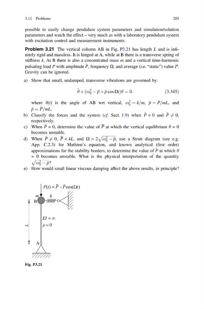
Problem 3.21 The vertical column AB in Fig. P3.21 has length L and is infinitely rigid and massless. It is hinged at A, while at B there is a transverse spring of
stiffness k. At B there is also a concentrated mass m and a vertical time-harmonic
pulsating load P with amplitude ~
P; frequency X, and average (i.e. “static”) value P:
Gravity can be ignored.
a) Show that small, undamped, transverse vibrations are governed by:
€ h þ ðx
2
0 À p þ ~ p cos XtÞh ¼ 0:
ð3:345Þ
where h(t) is the angle of AB wrt vertical, x
2
0 ¼ k=m, p ¼
P=mL, and
~ p ¼ ~
P=mL:
b) Classify the forces and the system (cf. Sect. 1.9) when ~
P = 0 and ~
P 6 ¼ 0,
respectively.
c) When ~
P = 0, determine the value of P at which the vertical equilibrium h = 0
becomes unstable.
d) When ~
P 6 ¼ 0, P < kL, and X [ 2
ffiffiffiffiffiffiffiffiffiffiffiffiffiffi
x 2
0 À p
p
, use a Strutt diagram (see e.g.
App. C.2.3) for Mathieu’s equation, and known analytical (first order)
approximations for the stability borders, to determine the value of ~
P at which h
= 0 becomes unstable. What is the physical interpretation of the quantity
ffiffiffiffiffiffiffiffiffiffiffiffiffiffi
x 2
0 À p
p
?
e) How would small linear viscous damping affect the above results, in principle?
Fig. P3.21
3.11 Problems
205
parameters and watch the effect – very much as with a laboratory pendulum system
with excitation control and measurement instruments.
Problem 3.21 The vertical column AB in Fig. P3.21 has length L and is infinitely rigid and massless. It is hinged at A, while at B there is a transverse spring of
stiffness k. At B there is also a concentrated mass m and a vertical time-harmonic
pulsating load P with amplitude ~
P; frequency X, and average (i.e. “static”) value P:
Gravity can be ignored.
a) Show that small, undamped, transverse vibrations are governed by:
€ h þ ðx
2
0 À p þ ~ p cos XtÞh ¼ 0:
ð3:345Þ
where h(t) is the angle of AB wrt vertical, x
2
0 ¼ k=m, p ¼
P=mL, and
~ p ¼ ~
P=mL:
b) Classify the forces and the system (cf. Sect. 1.9) when ~
P = 0 and ~
P 6 ¼ 0,
respectively.
c) When ~
P = 0, determine the value of P at which the vertical equilibrium h = 0
becomes unstable.
d) When ~
P 6 ¼ 0, P < kL, and X [ 2
ffiffiffiffiffiffiffiffiffiffiffiffiffiffi
x 2
0 À p
p
, use a Strutt diagram (see e.g.
App. C.2.3) for Mathieu’s equation, and known analytical (first order)
approximations for the stability borders, to determine the value of ~
P at which h
= 0 becomes unstable. What is the physical interpretation of the quantity
ffiffiffiffiffiffiffiffiffiffiffiffiffiffi
x 2
0 À p
p
?
e) How would small linear viscous damping affect the above results, in principle?
Fig. P3.21
3.11 Problems
205