

s ¼
2D
p
PðzÞ;
ð3:297Þ
with P defined by (3.274). Inserting this into (3.296) gives:
€ z þ M z
ð ÞP z
ð Þ ¼ Àh 1 _
z À h 2 _
z
2 M z
ð Þ À h 3 _
z
3
for z 6 ¼
p
2
þ jp; j ¼ 0; 1; . . .;
_
z þ À _
z À ¼ À 1 À R
ð
Þ_ z À for z ¼
p
2
þ jp;
ð3:298Þ
where h 1 ¼ h 1 ; h 2 ¼ 2Dh 2 /p; h 3 ¼ 4D
2 h 3 =p
2
; and M(z) = dP/dz. We assume a
small energy input (corresponding to a small negative slope of the friction characteristics), and small energy dissipation due to friction and impact, i.e.:
0\ ð1 À RÞ ( 1; h 1;2;3
( 1; D ¼ Oð1Þ:
ð3:299Þ
Next we should transform (3.298) into the general form (3.258) applicable for
averaging. But contrary to the one-sided oscillator of Sect. 3.9.5, the van der Pol
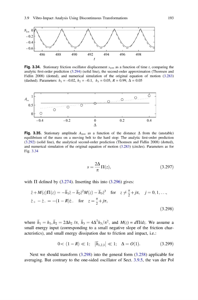
Fig. 3.34. Stationary friction oscillator displacement s 1∞ as a function of time t, comparing the
analytic first-order prediction (3.294) (solid line), the second-order approximation (Thomsen and
Fidlin 2008) (dotted), and numerical simulation of the original equation of motion (3.283)
(dashed). Parameters: h 1 = –0.02, h 2 = –0.1, h 3 = 0.05, R = 0.99, D = 0.05
Fig. 3.35. Stationary amplitude A 1∞ as a function of the distance D from the (unstable)
equilibrium of the mass on a moving belt to the hard stop: The analytic first-order prediction
(3.292) (solid line), the analytical second-order prediction (Thomsen and Fidlin 2008) (dotted),
and numerical simulation of the original equation of motion (3.283) (circles). Parameters as for
Fig. 3.34
3.9 Vibro-Impact Analysis Using Discontinuous Transformations
193
2D
p
PðzÞ;
ð3:297Þ
with P defined by (3.274). Inserting this into (3.296) gives:
€ z þ M z
ð ÞP z
ð Þ ¼ Àh 1 _
z À h 2 _
z
2 M z
ð Þ À h 3 _
z
3
for z 6 ¼
p
2
þ jp; j ¼ 0; 1; . . .;
_
z þ À _
z À ¼ À 1 À R
ð
Þ_ z À for z ¼
p
2
þ jp;
ð3:298Þ
where h 1 ¼ h 1 ; h 2 ¼ 2Dh 2 /p; h 3 ¼ 4D
2 h 3 =p
2
; and M(z) = dP/dz. We assume a
small energy input (corresponding to a small negative slope of the friction characteristics), and small energy dissipation due to friction and impact, i.e.:
0\ ð1 À RÞ ( 1; h 1;2;3
( 1; D ¼ Oð1Þ:
ð3:299Þ
Next we should transform (3.298) into the general form (3.258) applicable for
averaging. But contrary to the one-sided oscillator of Sect. 3.9.5, the van der Pol
Fig. 3.34. Stationary friction oscillator displacement s 1∞ as a function of time t, comparing the
analytic first-order prediction (3.294) (solid line), the second-order approximation (Thomsen and
Fidlin 2008) (dotted), and numerical simulation of the original equation of motion (3.283)
(dashed). Parameters: h 1 = –0.02, h 2 = –0.1, h 3 = 0.05, R = 0.99, D = 0.05
Fig. 3.35. Stationary amplitude A 1∞ as a function of the distance D from the (unstable)
equilibrium of the mass on a moving belt to the hard stop: The analytic first-order prediction
(3.292) (solid line), the analytical second-order prediction (Thomsen and Fidlin 2008) (dotted),
and numerical simulation of the original equation of motion (3.283) (circles). Parameters as for
Fig. 3.34
3.9 Vibro-Impact Analysis Using Discontinuous Transformations
193