

which are to be employed in subsequent chapters. Finally some additional aids
useful in vibration analysis are described: Nondimensionalizing equations of
motion, relating various types and measures of damping, and deriving equations of
motions using the flexibility and stiffness methods.
1.2 Single Degree of Freedom Systems
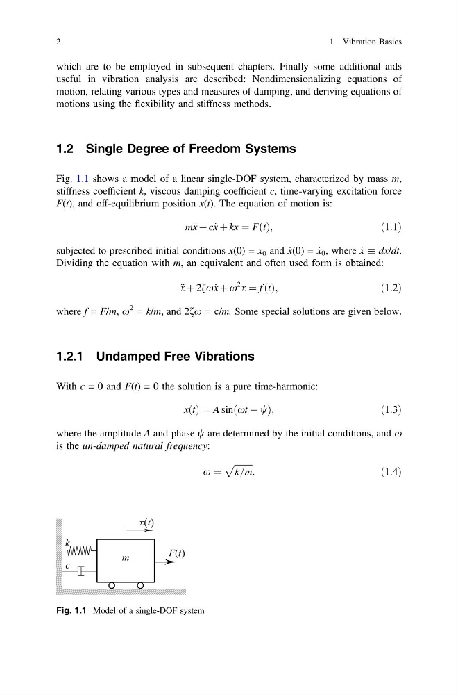
Fig. 1.1 shows a model of a linear single-DOF system, characterized by mass m,
stiffness coefficient k, viscous damping coefficient c, time-varying excitation force
F(t), and off-equilibrium position x(t). The equation of motion is:
m€ x þ c_ x þ kx ¼ FðtÞ;
ð1:1Þ
subjected to prescribed initial conditions x(0) = x 0 and _
x(0) = _
x 0 , where _
x dx/dt.
Dividing the equation with m, an equivalent and often used form is obtained:
€ x þ 2fx_ x þ x
2 x ¼ f ðtÞ;
ð1:2Þ
where f = F/m, x
2 = k/m, and 2fx = c/m. Some special solutions are given below.
1.2.1 Undamped Free Vibrations
With c = 0 and F(t) = 0 the solution is a pure time-harmonic:
xðtÞ ¼ A sinðxt À wÞ;
ð1:3Þ
where the amplitude A and phase w are determined by the initial conditions, and x
is the un-damped natural frequency:
x ¼
ffiffiffiffiffiffiffiffi ffi
k=m
p
:
ð1:4Þ
x t
( )
k
c
m
F t
( )
Fig. 1.1 Model of a single-DOF system
2
1 Vibration Basics
useful in vibration analysis are described: Nondimensionalizing equations of
motion, relating various types and measures of damping, and deriving equations of
motions using the flexibility and stiffness methods.
1.2 Single Degree of Freedom Systems
Fig. 1.1 shows a model of a linear single-DOF system, characterized by mass m,
stiffness coefficient k, viscous damping coefficient c, time-varying excitation force
F(t), and off-equilibrium position x(t). The equation of motion is:
m€ x þ c_ x þ kx ¼ FðtÞ;
ð1:1Þ
subjected to prescribed initial conditions x(0) = x 0 and _
x(0) = _
x 0 , where _
x dx/dt.
Dividing the equation with m, an equivalent and often used form is obtained:
€ x þ 2fx_ x þ x
2 x ¼ f ðtÞ;
ð1:2Þ
where f = F/m, x
2 = k/m, and 2fx = c/m. Some special solutions are given below.
1.2.1 Undamped Free Vibrations
With c = 0 and F(t) = 0 the solution is a pure time-harmonic:
xðtÞ ¼ A sinðxt À wÞ;
ð1:3Þ
where the amplitude A and phase w are determined by the initial conditions, and x
is the un-damped natural frequency:
x ¼
ffiffiffiffiffiffiffiffi ffi
k=m
p
:
ð1:4Þ
x t
( )
k
c
m
F t
( )
Fig. 1.1 Model of a single-DOF system
2
1 Vibration Basics