

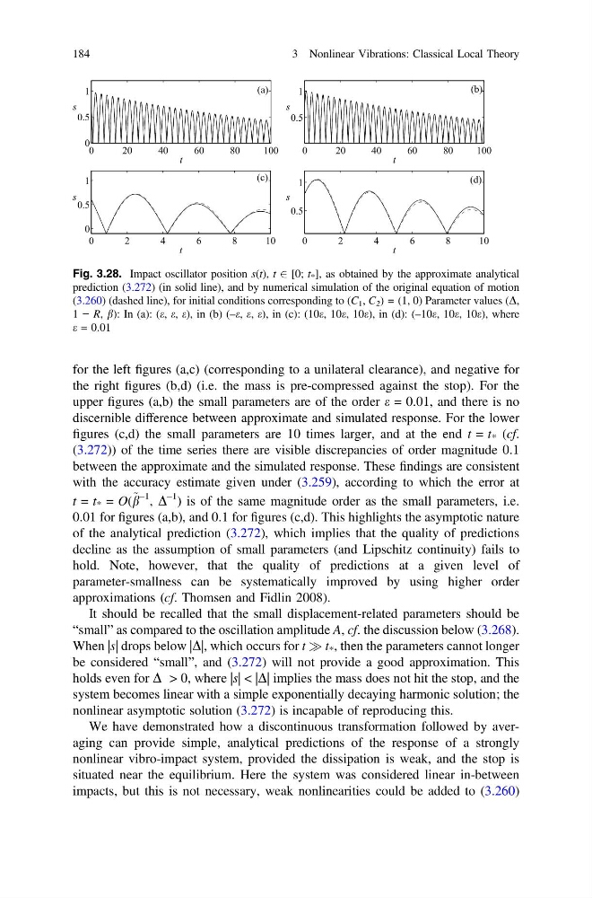
for the left figures (a,c) (corresponding to a unilateral clearance), and negative for
the right figures (b,d) (i.e. the mass is pre-compressed against the stop). For the
upper figures (a,b) the small parameters are of the order e = 0.01, and there is no
discernible difference between approximate and simulated response. For the lower
figures (c,d) the small parameters are 10 times larger, and at the end t = t * (cf.
(3.272)) of the time series there are visible discrepancies of order magnitude 0.1
between the approximate and the simulated response. These findings are consistent
with the accuracy estimate given under (3.259), according to which the error at
t = t * = O( ~
b
–1 , D
–1 ) is of the same magnitude order as the small parameters, i.e.
0.01 for figures (a,b), and 0.1 for figures (c,d). This highlights the asymptotic nature
of the analytical prediction (3.272), which implies that the quality of predictions
decline as the assumption of small parameters (and Lipschitz continuity) fails to
hold. Note, however, that the quality of predictions at a given level of
parameter-smallness can be systematically improved by using higher order
approximations (cf. Thomsen and Fidlin 2008).
It should be recalled that the small displacement-related parameters should be
“small” as compared to the oscillation amplitude A, cf. the discussion below (3.268).
When |s| drops below |D|, which occurs for t ) t * , then the parameters cannot longer
be considered “small”, and (3.272) will not provide a good approximation. This
holds even for D > 0, where |s| < |D| implies the mass does not hit the stop, and the
system becomes linear with a simple exponentially decaying harmonic solution; the
nonlinear asymptotic solution (3.272) is incapable of reproducing this.
We have demonstrated how a discontinuous transformation followed by averaging can provide simple, analytical predictions of the response of a strongly
nonlinear vibro-impact system, provided the dissipation is weak, and the stop is
situated near the equilibrium. Here the system was considered linear in-between
impacts, but this is not necessary, weak nonlinearities could be added to (3.260)
Fig. 3.28. Impact oscillator position s(t), t 2 [0; t * ], as obtained by the approximate analytical
prediction (3.272) (in solid line), and by numerical simulation of the original equation of motion
(3.260) (dashed line), for initial conditions corresponding to (C 1 , C 2 ) = (1, 0) Parameter values (D,
1 − R, b): In (a): (e, e, e), in (b) (–e, e, e), in (c): (10e, 10e, 10e), in (d): (–10e, 10e, 10e), where
e = 0.01
184
3 Nonlinear Vibrations: Classical Local Theory
the right figures (b,d) (i.e. the mass is pre-compressed against the stop). For the
upper figures (a,b) the small parameters are of the order e = 0.01, and there is no
discernible difference between approximate and simulated response. For the lower
figures (c,d) the small parameters are 10 times larger, and at the end t = t * (cf.
(3.272)) of the time series there are visible discrepancies of order magnitude 0.1
between the approximate and the simulated response. These findings are consistent
with the accuracy estimate given under (3.259), according to which the error at
t = t * = O( ~
b
–1 , D
–1 ) is of the same magnitude order as the small parameters, i.e.
0.01 for figures (a,b), and 0.1 for figures (c,d). This highlights the asymptotic nature
of the analytical prediction (3.272), which implies that the quality of predictions
decline as the assumption of small parameters (and Lipschitz continuity) fails to
hold. Note, however, that the quality of predictions at a given level of
parameter-smallness can be systematically improved by using higher order
approximations (cf. Thomsen and Fidlin 2008).
It should be recalled that the small displacement-related parameters should be
“small” as compared to the oscillation amplitude A, cf. the discussion below (3.268).
When |s| drops below |D|, which occurs for t ) t * , then the parameters cannot longer
be considered “small”, and (3.272) will not provide a good approximation. This
holds even for D > 0, where |s| < |D| implies the mass does not hit the stop, and the
system becomes linear with a simple exponentially decaying harmonic solution; the
nonlinear asymptotic solution (3.272) is incapable of reproducing this.
We have demonstrated how a discontinuous transformation followed by averaging can provide simple, analytical predictions of the response of a strongly
nonlinear vibro-impact system, provided the dissipation is weak, and the stop is
situated near the equilibrium. Here the system was considered linear in-between
impacts, but this is not necessary, weak nonlinearities could be added to (3.260)
Fig. 3.28. Impact oscillator position s(t), t 2 [0; t * ], as obtained by the approximate analytical
prediction (3.272) (in solid line), and by numerical simulation of the original equation of motion
(3.260) (dashed line), for initial conditions corresponding to (C 1 , C 2 ) = (1, 0) Parameter values (D,
1 − R, b): In (a): (e, e, e), in (b) (–e, e, e), in (c): (10e, 10e, 10e), in (d): (–10e, 10e, 10e), where
e = 0.01
184
3 Nonlinear Vibrations: Classical Local Theory