

2bx 0 X
ð
Þ
2 þ X
2
À x
2
0
À
Á À
3
4
ca
2
2
!
a
2
¼ q
2
;
tan u ¼
À X
2
À x
2
0
À
Á þ
3
8 ca
2
2bxX
;
ð3:242Þ
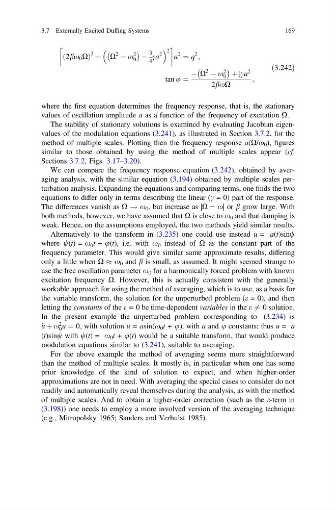
where the first equation determines the frequency response, that is, the stationary
values of oscillation amplitude a as a function of the frequency of excitation X.
The stability of stationary solutions is examined by evaluating Jacobian eigenvalues of the modulation equations (3.241), as illustrated in Section 3.7.2. for the
method of multiple scales. Plotting then the frequency response a(X/x 0 ), figures
similar to those obtained by using the method of multiple scales appear (cf.
Sections 3.7.2, Figs. 3.17–3.20).
We can compare the frequency response equation (3.242), obtained by averaging analysis, with the similar equation (3.194) obtained by multiple scales perturbation analysis. Expanding the equations and comparing terms, one finds the two
equations to differ only in terms describing the linear (c = 0) part of the response.
The differences vanish as X ! x 0 , but increase as |X − x| or b grow large. With
both methods, however, we have assumed that X is close to x 0 and that damping is
weak. Hence, on the assumptions employed, the two methods yield similar results.
Alternatively to the transform in (3.235) one could use instead u = a(t)sinw
where w(t) = x 0 t + u(t), i.e. with x 0 instead of X as the constant part of the
frequency parameter. This would give similar same approximate results, differing
only a little when X % x 0 and b is small, as assumed. It might seemed strange to
use the free oscillation parameter x 0 for a harmonically forced problem with known
excitation frequency X. However, this is actually consistent with the generally
workable approach for using the method of averaging, which is to use, as a basis for
the variable transform, the solution for the unperturbed problem (e = 0), and then
letting the constants of the e = 0 be time-dependent variables in the e 6 ¼ 0 solution.
In the present example the unperturbed problem corresponding to (3.234) is
€ u þ x
2
0 u ¼ 0; with solution u = asin(x 0 t + u), with a and u constants; thus u = a
(t)sinw with w(t) = x 0 t + u(t) would be a suitable transform, that would produce
modulation equations similar to (3.241), suitable to averaging.
For the above example the method of averaging seems more straightforward
than the method of multiple scales. It mostly is, in particular when one has some
prior knowledge of the kind of solution to expect, and when higher-order
approximations are not in need. With averaging the special cases to consider do not
readily and automatically reveal themselves during the analysis, as with the method
of multiple scales. And to obtain a higher-order correction (such as the e-term in
(3.198)) one needs to employ a more involved version of the averaging technique
(e.g., Mitropolsky 1965; Sanders and Verhulst 1985).
3.7 Externally Excited Duffing Systems
169
ð
Þ
2 þ X
2
À x
2
0
À
Á À
3
4
ca
2
2
!
a
2
¼ q
2
;
tan u ¼
À X
2
À x
2
0
À
Á þ
3
8 ca
2
2bxX
;
ð3:242Þ
where the first equation determines the frequency response, that is, the stationary
values of oscillation amplitude a as a function of the frequency of excitation X.
The stability of stationary solutions is examined by evaluating Jacobian eigenvalues of the modulation equations (3.241), as illustrated in Section 3.7.2. for the
method of multiple scales. Plotting then the frequency response a(X/x 0 ), figures
similar to those obtained by using the method of multiple scales appear (cf.
Sections 3.7.2, Figs. 3.17–3.20).
We can compare the frequency response equation (3.242), obtained by averaging analysis, with the similar equation (3.194) obtained by multiple scales perturbation analysis. Expanding the equations and comparing terms, one finds the two
equations to differ only in terms describing the linear (c = 0) part of the response.
The differences vanish as X ! x 0 , but increase as |X − x| or b grow large. With
both methods, however, we have assumed that X is close to x 0 and that damping is
weak. Hence, on the assumptions employed, the two methods yield similar results.
Alternatively to the transform in (3.235) one could use instead u = a(t)sinw
where w(t) = x 0 t + u(t), i.e. with x 0 instead of X as the constant part of the
frequency parameter. This would give similar same approximate results, differing
only a little when X % x 0 and b is small, as assumed. It might seemed strange to
use the free oscillation parameter x 0 for a harmonically forced problem with known
excitation frequency X. However, this is actually consistent with the generally
workable approach for using the method of averaging, which is to use, as a basis for
the variable transform, the solution for the unperturbed problem (e = 0), and then
letting the constants of the e = 0 be time-dependent variables in the e 6 ¼ 0 solution.
In the present example the unperturbed problem corresponding to (3.234) is
€ u þ x
2
0 u ¼ 0; with solution u = asin(x 0 t + u), with a and u constants; thus u = a
(t)sinw with w(t) = x 0 t + u(t) would be a suitable transform, that would produce
modulation equations similar to (3.241), suitable to averaging.
For the above example the method of averaging seems more straightforward
than the method of multiple scales. It mostly is, in particular when one has some
prior knowledge of the kind of solution to expect, and when higher-order
approximations are not in need. With averaging the special cases to consider do not
readily and automatically reveal themselves during the analysis, as with the method
of multiple scales. And to obtain a higher-order correction (such as the e-term in
(3.198)) one needs to employ a more involved version of the averaging technique
(e.g., Mitropolsky 1965; Sanders and Verhulst 1985).
3.7 Externally Excited Duffing Systems
169