

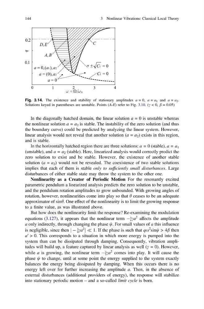
Fig. 3.14. The existence and stability of stationary amplitudes a = 0, a = a 1 and a = a 2 .
Solutions keyed in parentheses are unstable. Points (A-E) refer to Fig. 3.10. (c < 0, b = 0.05)
In the diagonally hatched domain, the linear solution a = 0 is unstable whereas
the nonlinear solution a = a 2 is stable. The instability of the zero solution (and thus
the boundary curve) could be predicted by analyzing the linear system. However,
linear analysis would not reveal that another solution (a = a 2 ) exists in this region,
and is stable.
In the horizontally hatched region there are three solutions: a = 0 (stable), a = a 1
(unstable), and a = a 2 (stable). Here, linearized analysis would correctly predict the
zero solution to exist and be stable. However, the existence of another stable
solution (a = a 2 ) would not be revealed. The coexistence of two stable solutions
implies that each of them is stable only to sufficiently small disturbances. Large
disturbances of either stable state may throw the system to the other one.
Nonlinearity as a Creator of Periodic Motion For the resonantly excited
parametric pendulum a linearized analysis predicts the zero solution to be unstable,
and the pendulum rotation amplitudes to grow unbounded. With growing angles of
rotation, however, nonlinearities come into play so that h ceases to be an adequate
approximator of sinh. One effect of the nonlinearity is to limit the growing response
to a finite value, as was illustrated above.
But how does the nonlinearity limit the response? Re-examining the modulation
equations (3.127), it appears that the nonlinear term À
3
4 ca
2 affects the amplitude
a only indirectly, through changing the phase w. For small values of a this influence
is negligible, since then j À
3
4 ca
2
j ( 1: If the phase is such that qx
2 sinw > 4b then
a′ > 0. This corresponds to a situation in which more energy is pumped into the
system than can be dissipated through damping. Consequently, vibration amplitudes will build up, a feature captured by linear analysis as well (c = 0). However,
while a is growing, the nonlinear term À
3
4 ca
2 comes into play. It will cause the
phase w to change, until at some point the energy supplied to the system exactly
balances the energy being dissipated by damping. When this occurs there is no
energy left over for further increasing the amplitude a. Then, in the absence of
external disturbances (additional providers of energy), the response will stabilize
into stationary periodic motion – and a so-called limit cycle is born.
144
3 Nonlinear Vibrations: Classical Local Theory
Solutions keyed in parentheses are unstable. Points (A-E) refer to Fig. 3.10. (c < 0, b = 0.05)
In the diagonally hatched domain, the linear solution a = 0 is unstable whereas
the nonlinear solution a = a 2 is stable. The instability of the zero solution (and thus
the boundary curve) could be predicted by analyzing the linear system. However,
linear analysis would not reveal that another solution (a = a 2 ) exists in this region,
and is stable.
In the horizontally hatched region there are three solutions: a = 0 (stable), a = a 1
(unstable), and a = a 2 (stable). Here, linearized analysis would correctly predict the
zero solution to exist and be stable. However, the existence of another stable
solution (a = a 2 ) would not be revealed. The coexistence of two stable solutions
implies that each of them is stable only to sufficiently small disturbances. Large
disturbances of either stable state may throw the system to the other one.
Nonlinearity as a Creator of Periodic Motion For the resonantly excited
parametric pendulum a linearized analysis predicts the zero solution to be unstable,
and the pendulum rotation amplitudes to grow unbounded. With growing angles of
rotation, however, nonlinearities come into play so that h ceases to be an adequate
approximator of sinh. One effect of the nonlinearity is to limit the growing response
to a finite value, as was illustrated above.
But how does the nonlinearity limit the response? Re-examining the modulation
equations (3.127), it appears that the nonlinear term À
3
4 ca
2 affects the amplitude
a only indirectly, through changing the phase w. For small values of a this influence
is negligible, since then j À
3
4 ca
2
j ( 1: If the phase is such that qx
2 sinw > 4b then
a′ > 0. This corresponds to a situation in which more energy is pumped into the
system than can be dissipated through damping. Consequently, vibration amplitudes will build up, a feature captured by linear analysis as well (c = 0). However,
while a is growing, the nonlinear term À
3
4 ca
2 comes into play. It will cause the
phase w to change, until at some point the energy supplied to the system exactly
balances the energy being dissipated by damping. When this occurs there is no
energy left over for further increasing the amplitude a. Then, in the absence of
external disturbances (additional providers of energy), the response will stabilize
into stationary periodic motion – and a so-called limit cycle is born.
144
3 Nonlinear Vibrations: Classical Local Theory