

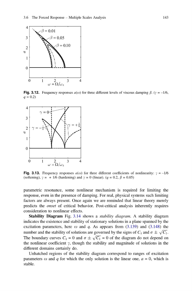
Fig. 3.12. Frequency responses a(x) for three different levels of viscous damping b. (c = –1/6,
q = 0.2)
Fig. 3.13. Frequency responses a(x) for three different coefficients of nonlinearity: c = –1/6
(softening), c = + 1/6 (hardening) and c = 0 (linear). (q = 0.2, b = 0.05)
parametric resonance, some nonlinear mechanism is required for limiting the
response, even in the presence of damping. For real, physical systems such limiting
factors are always present. Once again we are reminded that linear theory merely
predicts the onset of critical behavior. Post-critical analysis inherently requires
consideration to nonlinear effects.
Stability Diagram Fig. 3.14 shows a stability diagram. A stability diagram
indicates the existence and stability of stationary solutions in a plane spanned by the
excitation parameters, here x and q. As appears from (3.139) and (3.148) the
number and the stability of solutions are governed by the signs of C 1 and r ±
ffiffiffiffiffi ffi
C 1
p :
The boundary curves C 1 = 0 and r ±
ffiffiffiffiffi ffi
C 1
p
= 0 of the diagram do not depend on
the nonlinear coefficient c, though the stability and magnitude of solutions in the
different domains certainly do.
Unhatched regions of the stability diagram correspond to ranges of excitation
parameters x and q for which the only solution is the linear one, a = 0, which is
stable.
3.6 The Forced Response – Multiple Scales Analysis
143
q = 0.2)
Fig. 3.13. Frequency responses a(x) for three different coefficients of nonlinearity: c = –1/6
(softening), c = + 1/6 (hardening) and c = 0 (linear). (q = 0.2, b = 0.05)
parametric resonance, some nonlinear mechanism is required for limiting the
response, even in the presence of damping. For real, physical systems such limiting
factors are always present. Once again we are reminded that linear theory merely
predicts the onset of critical behavior. Post-critical analysis inherently requires
consideration to nonlinear effects.
Stability Diagram Fig. 3.14 shows a stability diagram. A stability diagram
indicates the existence and stability of stationary solutions in a plane spanned by the
excitation parameters, here x and q. As appears from (3.139) and (3.148) the
number and the stability of solutions are governed by the signs of C 1 and r ±
ffiffiffiffiffi ffi
C 1
p :
The boundary curves C 1 = 0 and r ±
ffiffiffiffiffi ffi
C 1
p
= 0 of the diagram do not depend on
the nonlinear coefficient c, though the stability and magnitude of solutions in the
different domains certainly do.
Unhatched regions of the stability diagram correspond to ranges of excitation
parameters x and q for which the only solution is the linear one, a = 0, which is
stable.
3.6 The Forced Response – Multiple Scales Analysis
143