

b
2
À C 2 [ 0 and À b þ
ffiffiffiffiffiffiffiffiffiffiffiffiffiffiffiffi
b
2
À C 2
q
[ 0;
ð3:145Þ
which is fulfilled (for b > 0) if and only if:
C 2 \0:
ð3:146Þ
For any softening nonlinearity one has c < 0 (recall that for the pendulum
c = À
1
6 ), and the condition for instability becomes, upon inserting (3.144):
3
4
c~ a
2
À r [ 0:
ð3:147Þ
For the two solutions ~ a = a 1 and ~ a = a 2 we obtain, by inserting (3.140):
3
4
c~ a
2
À r ¼
ðr þ
ffiffiffiffiffi ffi
C 1
p Þ À r ¼
ffiffiffiffiffi ffi
C 1
p [ 0for ~ a ¼ a 1 ;
ðr À
ffiffiffiffiffi ffi
C 1
p Þ À r ¼ À
ffiffiffiffiffi ffi
C 1
p \0for ~ a ¼ a 2 :
&
ð3:148Þ
Thus, by condition (3.147) we conclude that when c < 0 the a 1 -solution is
unstable, whereas the a 2 -solution is stable. (Conversely, for a hardening nonlinearity c > 0, the a 1 -solution is stable whereas the a 2 -solution is unstable).
3.6.6 Discussing Stationary Responses
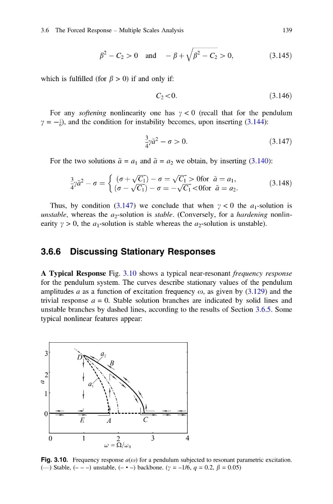
A Typical Response Fig. 3.10 shows a typical near-resonant frequency response
for the pendulum system. The curves describe stationary values of the pendulum
amplitudes a as a function of excitation frequency x, as given by (3.129) and the
trivial response a = 0. Stable solution branches are indicated by solid lines and
unstable branches by dashed lines, according to the results of Section 3.6.5. Some
typical nonlinear features appear:
Fig. 3.10. Frequency response a(x) for a pendulum subjected to resonant parametric excitation.
(—) Stable, (– – –) unstable, (– • –) backbone. (c = –1/6, q = 0.2, b = 0.05)
3.6 The Forced Response – Multiple Scales Analysis
139
2
À C 2 [ 0 and À b þ
ffiffiffiffiffiffiffiffiffiffiffiffiffiffiffiffi
b
2
À C 2
q
[ 0;
ð3:145Þ
which is fulfilled (for b > 0) if and only if:
C 2 \0:
ð3:146Þ
For any softening nonlinearity one has c < 0 (recall that for the pendulum
c = À
1
6 ), and the condition for instability becomes, upon inserting (3.144):
3
4
c~ a
2
À r [ 0:
ð3:147Þ
For the two solutions ~ a = a 1 and ~ a = a 2 we obtain, by inserting (3.140):
3
4
c~ a
2
À r ¼
ðr þ
ffiffiffiffiffi ffi
C 1
p Þ À r ¼
ffiffiffiffiffi ffi
C 1
p [ 0for ~ a ¼ a 1 ;
ðr À
ffiffiffiffiffi ffi
C 1
p Þ À r ¼ À
ffiffiffiffiffi ffi
C 1
p \0for ~ a ¼ a 2 :
&
ð3:148Þ
Thus, by condition (3.147) we conclude that when c < 0 the a 1 -solution is
unstable, whereas the a 2 -solution is stable. (Conversely, for a hardening nonlinearity c > 0, the a 1 -solution is stable whereas the a 2 -solution is unstable).
3.6.6 Discussing Stationary Responses
A Typical Response Fig. 3.10 shows a typical near-resonant frequency response
for the pendulum system. The curves describe stationary values of the pendulum
amplitudes a as a function of excitation frequency x, as given by (3.129) and the
trivial response a = 0. Stable solution branches are indicated by solid lines and
unstable branches by dashed lines, according to the results of Section 3.6.5. Some
typical nonlinear features appear:
Fig. 3.10. Frequency response a(x) for a pendulum subjected to resonant parametric excitation.
(—) Stable, (– – –) unstable, (– • –) backbone. (c = –1/6, q = 0.2, b = 0.05)
3.6 The Forced Response – Multiple Scales Analysis
139