

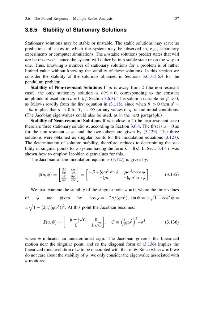
3.6.5 Stability of Stationary Solutions
Stationary solutions may be stable or unstable. The stable solutions may serve as
predictions of states in which the system may be observed in, e.g., laboratory
experiments or computer simulations. The unstable solutions predict states that will
not be observed – since the system will either be in a stable state or on the way to
one. Thus, knowing a number of stationary solutions for a problem is of rather
limited value without knowing the stability of these solutions. In this section we
consider the stability of the solutions obtained in Sections 3.6.3–3.6.4 for the
pendulum problem.
Stability of Non-resonant Solutions If x is away from 2 (the non-resonant
case), the only stationary solution is h(s) = 0, corresponding to the constant
amplitude of oscillation a = 0 (cf. Section 3.6.3). This solution is stable for b > 0,
as follows readily from the first equation in (3.118), since when b > 0 then a
0
¼
Àba implies that a ! 0 for T 1 ! ∞ for any values of q, x and initial conditions.
(The Jacobian eigenvalues could also be used, as in the next paragraph.)
Stability of Near-resonant Solutions If x is close to 2 (the near-resonant case)
there are three stationary solutions, according to Section 3.6.4. The first is a = 0 as
for the non-resonant case, and the two others are given by (3.129). The three
solutions were obtained as singular points for the modulation equations (3.127).
The determination of solution stability, therefore, reduces to determining the stability of singular points for a system having the form _
x = f(x). In Sect. 3.4.4 it was
shown how to employ Jacobian eigenvalues for this.
The Jacobian of the modulation equations (3.127) is given by:
Jða; wÞ ¼
@a
0
@a
@a
0
@w
@w
0
@a
@w
0
@w
"
#
¼
Àb þ
1
4 qx
2 sin w
1
4 qx
2 a cos w
À
3
2 ca
À
1
2 qx
2 sin w
!
:
ð3:135Þ
We first examine the stability of the singular point a = 0, where the limit values
of
w
are
given
by
cos w ¼ À2r=ðqx
2
Þ; sin w ¼ Æ
ffiffiffiffiffiffiffiffiffiffiffiffiffiffiffiffiffiffiffiffiffi
1 À cos 2 w
p
¼
Æ
ffiffiffiffiffiffiffiffiffiffiffiffiffiffiffiffiffiffiffiffiffiffiffiffiffiffiffiffiffiffiffiffiffi
1 À ð2r=ðqx 2 ÞÞ
2
q
: At this point the Jacobian becomes:
Jða; wÞ ¼
Àb Æ
1
2
ffiffiffi ffi
C
p
0
0
Æ
ffiffiffi ffi
C
p
!
; C
1
2
qx
2
2 Àr
2
:
ð3:136Þ
where ± indicates an undetermined sign. The Jacobian governs the linearized
motion near the singular point, and so the diagonal form of (3.136) implies the
linearized time evolution of a to be uncoupled with that of w. Since when a = 0 we
do not care about the stability of w, we only consider the eigenvalue associated with
a-motions:
3.6 The Forced Response – Multiple Scales Analysis
137
Stationary solutions may be stable or unstable. The stable solutions may serve as
predictions of states in which the system may be observed in, e.g., laboratory
experiments or computer simulations. The unstable solutions predict states that will
not be observed – since the system will either be in a stable state or on the way to
one. Thus, knowing a number of stationary solutions for a problem is of rather
limited value without knowing the stability of these solutions. In this section we
consider the stability of the solutions obtained in Sections 3.6.3–3.6.4 for the
pendulum problem.
Stability of Non-resonant Solutions If x is away from 2 (the non-resonant
case), the only stationary solution is h(s) = 0, corresponding to the constant
amplitude of oscillation a = 0 (cf. Section 3.6.3). This solution is stable for b > 0,
as follows readily from the first equation in (3.118), since when b > 0 then a
0
¼
Àba implies that a ! 0 for T 1 ! ∞ for any values of q, x and initial conditions.
(The Jacobian eigenvalues could also be used, as in the next paragraph.)
Stability of Near-resonant Solutions If x is close to 2 (the near-resonant case)
there are three stationary solutions, according to Section 3.6.4. The first is a = 0 as
for the non-resonant case, and the two others are given by (3.129). The three
solutions were obtained as singular points for the modulation equations (3.127).
The determination of solution stability, therefore, reduces to determining the stability of singular points for a system having the form _
x = f(x). In Sect. 3.4.4 it was
shown how to employ Jacobian eigenvalues for this.
The Jacobian of the modulation equations (3.127) is given by:
Jða; wÞ ¼
@a
0
@a
@a
0
@w
@w
0
@a
@w
0
@w
"
#
¼
Àb þ
1
4 qx
2 sin w
1
4 qx
2 a cos w
À
3
2 ca
À
1
2 qx
2 sin w
!
:
ð3:135Þ
We first examine the stability of the singular point a = 0, where the limit values
of
w
are
given
by
cos w ¼ À2r=ðqx
2
Þ; sin w ¼ Æ
ffiffiffiffiffiffiffiffiffiffiffiffiffiffiffiffiffiffiffiffiffi
1 À cos 2 w
p
¼
Æ
ffiffiffiffiffiffiffiffiffiffiffiffiffiffiffiffiffiffiffiffiffiffiffiffiffiffiffiffiffiffiffiffiffi
1 À ð2r=ðqx 2 ÞÞ
2
q
: At this point the Jacobian becomes:
Jða; wÞ ¼
Àb Æ
1
2
ffiffiffi ffi
C
p
0
0
Æ
ffiffiffi ffi
C
p
!
; C
1
2
qx
2
2 Àr
2
:
ð3:136Þ
where ± indicates an undetermined sign. The Jacobian governs the linearized
motion near the singular point, and so the diagonal form of (3.136) implies the
linearized time evolution of a to be uncoupled with that of w. Since when a = 0 we
do not care about the stability of w, we only consider the eigenvalue associated with
a-motions:
3.6 The Forced Response – Multiple Scales Analysis
137