

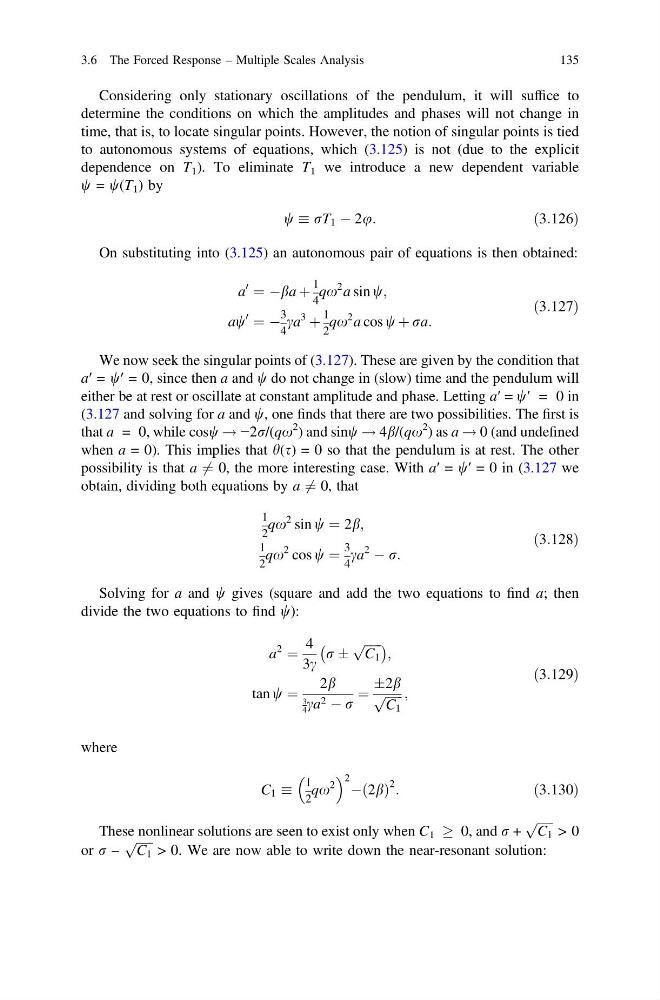
Considering only stationary oscillations of the pendulum, it will suffice to
determine the conditions on which the amplitudes and phases will not change in
time, that is, to locate singular points. However, the notion of singular points is tied
to autonomous systems of equations, which (3.125) is not (due to the explicit
dependence on T 1 ). To eliminate T 1 we introduce a new dependent variable
w = w(T 1 ) by
w rT 1 À 2u:
ð3:126Þ
On substituting into (3.125) an autonomous pair of equations is then obtained:
a
0
¼ Àba þ
1
4
qx
2 a sin w;
aw
0
¼ À
3
4
ca
3
þ
1
2
qx
2 a cos w þ ra:
ð3:127Þ
We now seek the singular points of (3.127). These are given by the condition that
a′ = w′ = 0, since then a and w do not change in (slow) time and the pendulum will
either be at rest or oscillate at constant amplitude and phase. Letting a′ = w′ = 0 in
(3.127 and solving for a and w, one finds that there are two possibilities. The first is
that a = 0, while cosw ! −2r/(qx
2 ) and sinw ! 4b/(qx
2 ) as a ! 0 (and undefined
when a = 0). This implies that h(s) = 0 so that the pendulum is at rest. The other
possibility is that a 6 ¼ 0, the more interesting case. With a′ = w′ = 0 in (3.127 we
obtain, dividing both equations by a 6 ¼ 0, that
1
2
qx
2 sin w ¼ 2b;
1
2
qx
2 cos w ¼
3
4
ca
2
À r:
ð3:128Þ
Solving for a and w gives (square and add the two equations to find a; then
divide the two equations to find w):
a
2
¼
4
3c
r Æ
ffiffiffiffiffi ffi
C 1
p
À
Á ;
tan w ¼
2b
3
4 ca 2 À r
¼
Æ2b
ffiffiffiffiffi ffi
C 1
p ;
ð3:129Þ
where
C 1
1
2
qx
2
2 À 2b
ð Þ
2 :
ð3:130Þ
These nonlinear solutions are seen to exist only when C 1 ! 0, and r +
ffiffiffiffiffi ffi
C 1
p
> 0
or r –
ffiffiffiffiffi ffi
C 1
p
> 0. We are now able to write down the near-resonant solution:
3.6 The Forced Response – Multiple Scales Analysis
135
determine the conditions on which the amplitudes and phases will not change in
time, that is, to locate singular points. However, the notion of singular points is tied
to autonomous systems of equations, which (3.125) is not (due to the explicit
dependence on T 1 ). To eliminate T 1 we introduce a new dependent variable
w = w(T 1 ) by
w rT 1 À 2u:
ð3:126Þ
On substituting into (3.125) an autonomous pair of equations is then obtained:
a
0
¼ Àba þ
1
4
qx
2 a sin w;
aw
0
¼ À
3
4
ca
3
þ
1
2
qx
2 a cos w þ ra:
ð3:127Þ
We now seek the singular points of (3.127). These are given by the condition that
a′ = w′ = 0, since then a and w do not change in (slow) time and the pendulum will
either be at rest or oscillate at constant amplitude and phase. Letting a′ = w′ = 0 in
(3.127 and solving for a and w, one finds that there are two possibilities. The first is
that a = 0, while cosw ! −2r/(qx
2 ) and sinw ! 4b/(qx
2 ) as a ! 0 (and undefined
when a = 0). This implies that h(s) = 0 so that the pendulum is at rest. The other
possibility is that a 6 ¼ 0, the more interesting case. With a′ = w′ = 0 in (3.127 we
obtain, dividing both equations by a 6 ¼ 0, that
1
2
qx
2 sin w ¼ 2b;
1
2
qx
2 cos w ¼
3
4
ca
2
À r:
ð3:128Þ
Solving for a and w gives (square and add the two equations to find a; then
divide the two equations to find w):
a
2
¼
4
3c
r Æ
ffiffiffiffiffi ffi
C 1
p
À
Á ;
tan w ¼
2b
3
4 ca 2 À r
¼
Æ2b
ffiffiffiffiffi ffi
C 1
p ;
ð3:129Þ
where
C 1
1
2
qx
2
2 À 2b
ð Þ
2 :
ð3:130Þ
These nonlinear solutions are seen to exist only when C 1 ! 0, and r +
ffiffiffiffiffi ffi
C 1
p
> 0
or r –
ffiffiffiffiffi ffi
C 1
p
> 0. We are now able to write down the near-resonant solution:
3.6 The Forced Response – Multiple Scales Analysis
135