

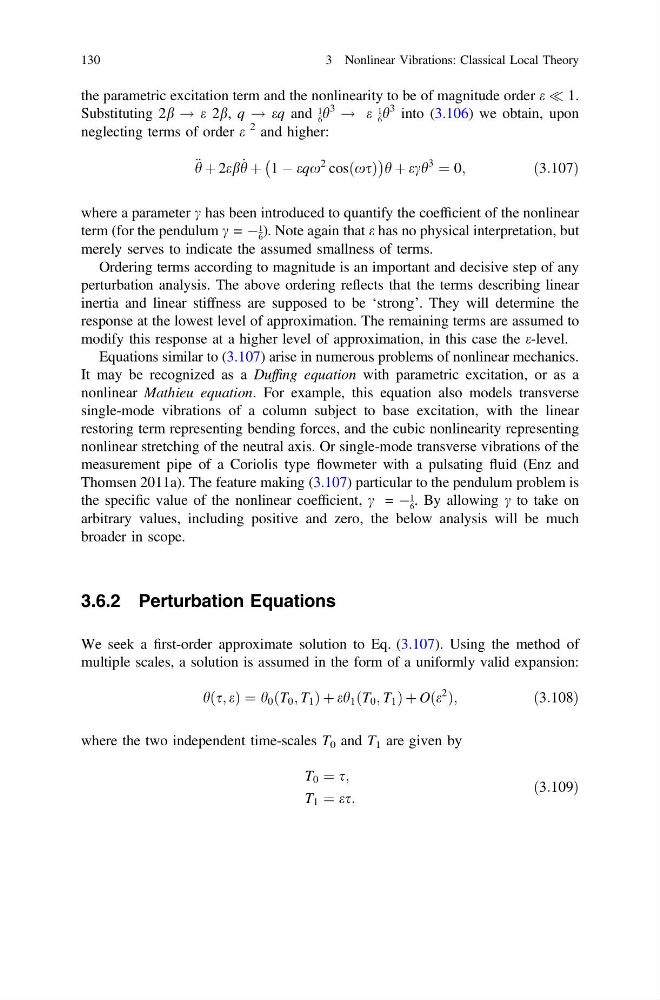
the parametric excitation term and the nonlinearity to be of magnitude order e ( 1.
Substituting 2b ! e 2b, q ! eq and
1
6 h
3
! e
1
6 h
3 into (3.106) we obtain, upon
neglecting terms of order e
2 and higher:
€ h þ 2eb _
h þ 1 À eqx
2 cosðxsÞ
À
Á
h þ ech
3
¼ 0;
ð3:107Þ
where a parameter c has been introduced to quantify the coefficient of the nonlinear
term (for the pendulum c = À
1
6 ). Note again that e has no physical interpretation, but
merely serves to indicate the assumed smallness of terms.
Ordering terms according to magnitude is an important and decisive step of any
perturbation analysis. The above ordering reflects that the terms describing linear
inertia and linear stiffness are supposed to be ‘strong’. They will determine the
response at the lowest level of approximation. The remaining terms are assumed to
modify this response at a higher level of approximation, in this case the e-level.
Equations similar to (3.107) arise in numerous problems of nonlinear mechanics.
It may be recognized as a Duffing equation with parametric excitation, or as a
nonlinear Mathieu equation. For example, this equation also models transverse
single-mode vibrations of a column subject to base excitation, with the linear
restoring term representing bending forces, and the cubic nonlinearity representing
nonlinear stretching of the neutral axis. Or single-mode transverse vibrations of the
measurement pipe of a Coriolis type flowmeter with a pulsating fluid (Enz and
Thomsen 2011a). The feature making (3.107) particular to the pendulum problem is
the specific value of the nonlinear coefficient, c = À
1
6 . By allowing c to take on
arbitrary values, including positive and zero, the below analysis will be much
broader in scope.
3.6.2 Perturbation Equations
We seek a first-order approximate solution to Eq. (3.107). Using the method of
multiple scales, a solution is assumed in the form of a uniformly valid expansion:
hðs; eÞ ¼ h 0 ðT 0 ; T 1 Þ þ eh 1 ðT 0 ; T 1 Þ þ Oðe
2
Þ;
ð3:108Þ
where the two independent time-scales T 0 and T 1 are given by
T 0 ¼ s;
T 1 ¼ es:
ð3:109Þ
130
3 Nonlinear Vibrations: Classical Local Theory
Substituting 2b ! e 2b, q ! eq and
1
6 h
3
! e
1
6 h
3 into (3.106) we obtain, upon
neglecting terms of order e
2 and higher:
€ h þ 2eb _
h þ 1 À eqx
2 cosðxsÞ
À
Á
h þ ech
3
¼ 0;
ð3:107Þ
where a parameter c has been introduced to quantify the coefficient of the nonlinear
term (for the pendulum c = À
1
6 ). Note again that e has no physical interpretation, but
merely serves to indicate the assumed smallness of terms.
Ordering terms according to magnitude is an important and decisive step of any
perturbation analysis. The above ordering reflects that the terms describing linear
inertia and linear stiffness are supposed to be ‘strong’. They will determine the
response at the lowest level of approximation. The remaining terms are assumed to
modify this response at a higher level of approximation, in this case the e-level.
Equations similar to (3.107) arise in numerous problems of nonlinear mechanics.
It may be recognized as a Duffing equation with parametric excitation, or as a
nonlinear Mathieu equation. For example, this equation also models transverse
single-mode vibrations of a column subject to base excitation, with the linear
restoring term representing bending forces, and the cubic nonlinearity representing
nonlinear stretching of the neutral axis. Or single-mode transverse vibrations of the
measurement pipe of a Coriolis type flowmeter with a pulsating fluid (Enz and
Thomsen 2011a). The feature making (3.107) particular to the pendulum problem is
the specific value of the nonlinear coefficient, c = À
1
6 . By allowing c to take on
arbitrary values, including positive and zero, the below analysis will be much
broader in scope.
3.6.2 Perturbation Equations
We seek a first-order approximate solution to Eq. (3.107). Using the method of
multiple scales, a solution is assumed in the form of a uniformly valid expansion:
hðs; eÞ ¼ h 0 ðT 0 ; T 1 Þ þ eh 1 ðT 0 ; T 1 Þ þ Oðe
2
Þ;
ð3:108Þ
where the two independent time-scales T 0 and T 1 are given by
T 0 ¼ s;
T 1 ¼ es:
ð3:109Þ
130
3 Nonlinear Vibrations: Classical Local Theory