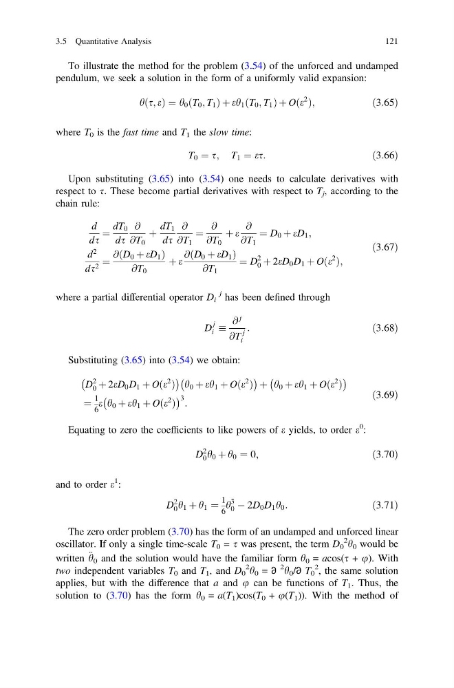
To illustrate the method for the problem (3.54) of the unforced and undamped
pendulum, we seek a solution in the form of a uniformly valid expansion:
hðs; eÞ ¼ h 0 ðT 0 ; T 1 Þ þ eh 1 ðT 0 ; T 1 Þ þ Oðe
2
Þ;
ð3:65Þ
where T 0 is the fast time and T 1 the slow time:
T 0 ¼ s; T 1 ¼ es:
ð3:66Þ
Upon substituting (3.65) into (3.54) one needs to calculate derivatives with
respect to s. These become partial derivatives with respect to T j , according to the
chain rule:
d
ds
¼
dT 0
ds
@
@T 0
þ
dT 1
ds
@
@T 1
¼
@
@T 0
þ e
@
@T 1
¼ D 0 þ eD 1 ;
d
2
ds 2 ¼
@ D 0 þ eD 1
ð
Þ
@T 0
þ e
@ D 0 þ eD 1
ð
Þ
@T 1
¼ D
2
0 þ 2eD 0 D 1 þ Oðe
2
Þ;
ð3:67Þ
where a partial differential operator D i
j has been defined through
D
j
i
@
j
@T
j
i
:
ð3:68Þ
Substituting (3.65) into (3.54) we obtain:
D
2
0 þ 2eD 0 D 1 þ Oðe
2
Þ
À
Á
h 0 þ eh 1 þ Oðe
2
Þ
À
Á þ h 0 þ eh 1 þ Oðe
2
Þ
À
Á
¼
1
6
e h 0 þ eh 1 þ Oðe
2
Þ
À
Á 3 :
ð3:69Þ
Equating to zero the coefficients to like powers of e yields, to order e
0 :
D
2
0 h 0 þ h 0 ¼ 0;
ð3:70Þ
and to order e
1 :
D
2
0 h 1 þ h 1 ¼
1
6
h
3
0 À 2D 0 D 1 h 0 :
ð3:71Þ
The zero order problem (3.70) has the form of an undamped and unforced linear
oscillator. If only a single time-scale T 0 = s was present, the term D 0
2
h 0 would be
written € h 0 and the solution would have the familiar form h 0 = acos(s + u). With
two independent variables T 0 and T 1 , and D 0
2 h 0 = ∂
2 h 0 /∂ T 0
2
, the same solution
applies, but with the difference that a and u can be functions of T 1 . Thus, the
solution to (3.70) has the form h 0 = a(T 1 )cos(T 0 + u(T 1 )). With the method of
3.5 Quantitative Analysis
121