

prove effective to most problems most of the time. Nayfeh (1973) offers a far more
complete discussion of perturbation methods than can be given here.
Little is lost by presenting the methods in terms of the pendulum example, so we
shall take this illustrative approach. For our purposes there is no reason to bother
about damping and forcing yet, so at this first stage we consider the equation of the
undamped and unforced pendulum (cf. (3.11)):
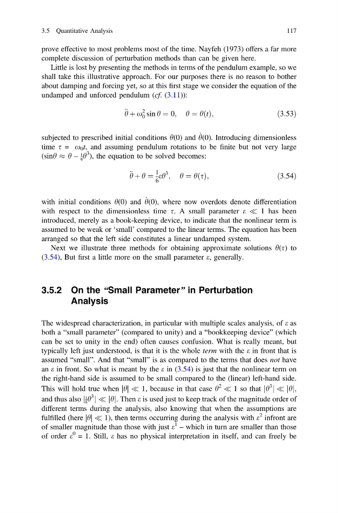
€ h þ x
2
0 sin h ¼ 0; h ¼ hðtÞ;
ð3:53Þ
subjected to prescribed initial conditions h(0) and _
h(0). Introducing dimensionless
time s = x 0 t, and assuming pendulum rotations to be finite but not very large
(sinh % h –
1
6 h
3 ), the equation to be solved becomes:
€ h þ h ¼
1
6
eh
3
; h ¼ hðsÞ;
ð3:54Þ
with initial conditions h(0) and _
h(0), where now overdots denote differentiation
with respect to the dimensionless time s. A small parameter e ( 1 has been
introduced, merely as a book-keeping device, to indicate that the nonlinear term is
assumed to be weak or ‘small’ compared to the linear terms. The equation has been
arranged so that the left side constitutes a linear undamped system.
Next we illustrate three methods for obtaining approximate solutions h(s) to
(3.54), But first a little more on the small parameter e, generally.
3.5.2 On the “Small Parameter” in Perturbation
Analysis
The widespread characterization, in particular with multiple scales analysis, of e as
both a “small parameter” (compared to unity) and a “bookkeeping device” (which
can be set to unity in the end) often causes confusion. What is really meant, but
typically left just understood, is that it is the whole term with the e in front that is
assumed “small”. And that “small” is as compared to the terms that does not have
an e in front. So what is meant by the e in (3.54) is just that the nonlinear term on
the right-hand side is assumed to be small compared to the (linear) left-hand side.
This will hold true when |h| ( 1, because in that case h
2
( 1 so that jh
3
j ( jhj;
and thus also j
1
6 h
3
j ( jhj: Then e is used just to keep track of the magnitude order of
different terms during the analysis, also knowing that when the assumptions are
fulfilled (here |h| ( 1), then terms occurring during the analysis with e
2 infront are
of smaller magnitude than those with just e
1
– which in turn are smaller than those
of order e
0 = 1. Still, e has no physical interpretation in itself, and can freely be
3.5 Quantitative Analysis
117
complete discussion of perturbation methods than can be given here.
Little is lost by presenting the methods in terms of the pendulum example, so we
shall take this illustrative approach. For our purposes there is no reason to bother
about damping and forcing yet, so at this first stage we consider the equation of the
undamped and unforced pendulum (cf. (3.11)):
€ h þ x
2
0 sin h ¼ 0; h ¼ hðtÞ;
ð3:53Þ
subjected to prescribed initial conditions h(0) and _
h(0). Introducing dimensionless
time s = x 0 t, and assuming pendulum rotations to be finite but not very large
(sinh % h –
1
6 h
3 ), the equation to be solved becomes:
€ h þ h ¼
1
6
eh
3
; h ¼ hðsÞ;
ð3:54Þ
with initial conditions h(0) and _
h(0), where now overdots denote differentiation
with respect to the dimensionless time s. A small parameter e ( 1 has been
introduced, merely as a book-keeping device, to indicate that the nonlinear term is
assumed to be weak or ‘small’ compared to the linear terms. The equation has been
arranged so that the left side constitutes a linear undamped system.
Next we illustrate three methods for obtaining approximate solutions h(s) to
(3.54), But first a little more on the small parameter e, generally.
3.5.2 On the “Small Parameter” in Perturbation
Analysis
The widespread characterization, in particular with multiple scales analysis, of e as
both a “small parameter” (compared to unity) and a “bookkeeping device” (which
can be set to unity in the end) often causes confusion. What is really meant, but
typically left just understood, is that it is the whole term with the e in front that is
assumed “small”. And that “small” is as compared to the terms that does not have
an e in front. So what is meant by the e in (3.54) is just that the nonlinear term on
the right-hand side is assumed to be small compared to the (linear) left-hand side.
This will hold true when |h| ( 1, because in that case h
2
( 1 so that jh
3
j ( jhj;
and thus also j
1
6 h
3
j ( jhj: Then e is used just to keep track of the magnitude order of
different terms during the analysis, also knowing that when the assumptions are
fulfilled (here |h| ( 1), then terms occurring during the analysis with e
2 infront are
of smaller magnitude than those with just e
1
– which in turn are smaller than those
of order e
0 = 1. Still, e has no physical interpretation in itself, and can freely be
3.5 Quantitative Analysis
117