

P ¼ a 1 a 2
½
:
ð3:39Þ
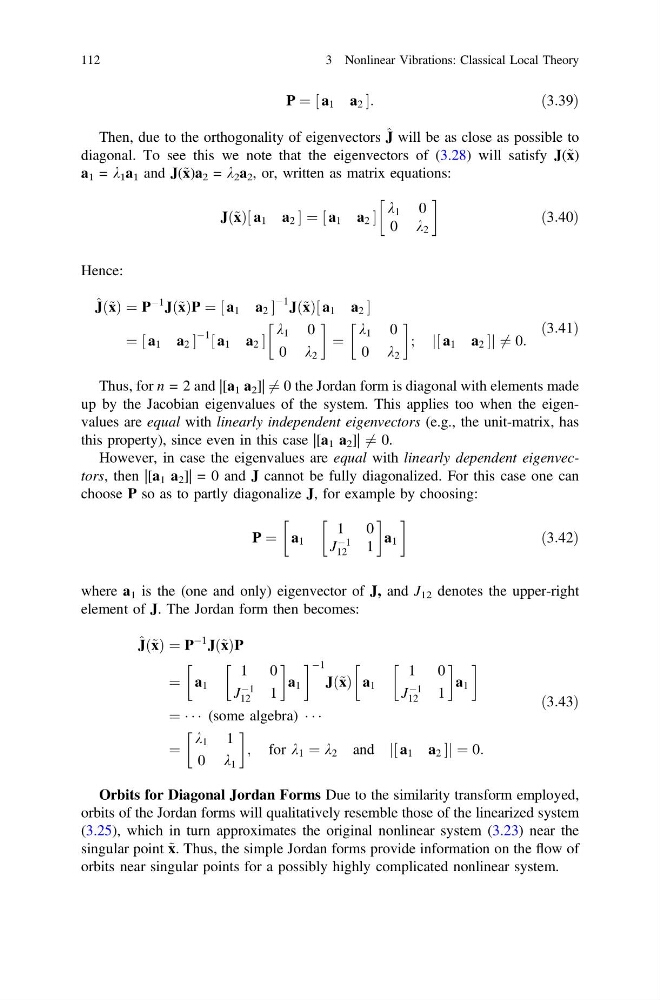
Then, due to the orthogonality of eigenvectors ^ J will be as close as possible to
diagonal. To see this we note that the eigenvectors of (3.28) will satisfy J(~ x)
a 1 = k 1 a 1 and J(~ x)a 2 = k 2 a 2 , or, written as matrix equations:
Jð~ xÞ a 1 a 2
½
¼ a 1 a 2
½
k 1 0
0 k 2
!
ð3:40Þ
Hence:
^ Jð~ xÞ ¼ P
À1
Jð~ xÞP ¼ a 1 a 2
½
À1 Jð~ xÞ a 1 a 2
½
¼ a 1 a 2
½
À1 a 1 a 2
½
k 1 0
0 k 2
!
¼
k 1 0
0 k 2
!
;
a 1 a 2
½
j
j6 ¼ 0:
ð3:41Þ
Thus, for n = 2 and |[a 1 a 2 ]| 6 ¼ 0 the Jordan form is diagonal with elements made
up by the Jacobian eigenvalues of the system. This applies too when the eigenvalues are equal with linearly independent eigenvectors (e.g., the unit-matrix, has
this property), since even in this case |[a 1 a 2 ]| 6 ¼ 0.
However, in case the eigenvalues are equal with linearly dependent eigenvectors, then |[a 1 a 2 ]| = 0 and J cannot be fully diagonalized. For this case one can
choose P so as to partly diagonalize J, for example by choosing:
P ¼ a 1
1 0
J
À1
12
1
!
a 1
!
ð3:42Þ
where a 1 is the (one and only) eigenvector of J, and J 12 denotes the upper-right
element of J. The Jordan form then becomes:
^ Jð~ xÞ ¼ P
À1
Jð~ xÞP
¼ a 1
1 0
J
À1
12
1
!
a 1
! À1
Jð~ xÞ a 1
1 0
J
À1
12
1
!
a 1
!
¼ Á Á Á (some algebra) Á Á Á
¼
k 1 1
0 k 1
!
; for k 1 ¼ k 2 and
a 1 a 2
½
j
j¼ 0:
ð3:43Þ
Orbits for Diagonal Jordan Forms Due to the similarity transform employed,
orbits of the Jordan forms will qualitatively resemble those of the linearized system
(3.25), which in turn approximates the original nonlinear system (3.23) near the
singular point ~ x. Thus, the simple Jordan forms provide information on the flow of
orbits near singular points for a possibly highly complicated nonlinear system.
112
3 Nonlinear Vibrations: Classical Local Theory
½
:
ð3:39Þ
Then, due to the orthogonality of eigenvectors ^ J will be as close as possible to
diagonal. To see this we note that the eigenvectors of (3.28) will satisfy J(~ x)
a 1 = k 1 a 1 and J(~ x)a 2 = k 2 a 2 , or, written as matrix equations:
Jð~ xÞ a 1 a 2
½
¼ a 1 a 2
½
k 1 0
0 k 2
!
ð3:40Þ
Hence:
^ Jð~ xÞ ¼ P
À1
Jð~ xÞP ¼ a 1 a 2
½
À1 Jð~ xÞ a 1 a 2
½
¼ a 1 a 2
½
À1 a 1 a 2
½
k 1 0
0 k 2
!
¼
k 1 0
0 k 2
!
;
a 1 a 2
½
j
j6 ¼ 0:
ð3:41Þ
Thus, for n = 2 and |[a 1 a 2 ]| 6 ¼ 0 the Jordan form is diagonal with elements made
up by the Jacobian eigenvalues of the system. This applies too when the eigenvalues are equal with linearly independent eigenvectors (e.g., the unit-matrix, has
this property), since even in this case |[a 1 a 2 ]| 6 ¼ 0.
However, in case the eigenvalues are equal with linearly dependent eigenvectors, then |[a 1 a 2 ]| = 0 and J cannot be fully diagonalized. For this case one can
choose P so as to partly diagonalize J, for example by choosing:
P ¼ a 1
1 0
J
À1
12
1
!
a 1
!
ð3:42Þ
where a 1 is the (one and only) eigenvector of J, and J 12 denotes the upper-right
element of J. The Jordan form then becomes:
^ Jð~ xÞ ¼ P
À1
Jð~ xÞP
¼ a 1
1 0
J
À1
12
1
!
a 1
! À1
Jð~ xÞ a 1
1 0
J
À1
12
1
!
a 1
!
¼ Á Á Á (some algebra) Á Á Á
¼
k 1 1
0 k 1
!
; for k 1 ¼ k 2 and
a 1 a 2
½
j
j¼ 0:
ð3:43Þ
Orbits for Diagonal Jordan Forms Due to the similarity transform employed,
orbits of the Jordan forms will qualitatively resemble those of the linearized system
(3.25), which in turn approximates the original nonlinear system (3.23) near the
singular point ~ x. Thus, the simple Jordan forms provide information on the flow of
orbits near singular points for a possibly highly complicated nonlinear system.
112
3 Nonlinear Vibrations: Classical Local Theory