

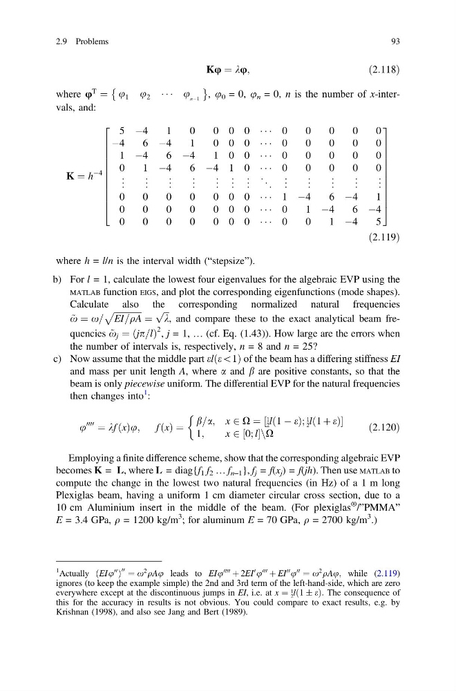
Ku ¼ ku;
ð2:118Þ
where u
T
¼ u 1 u 2 Á Á Á u nÀ1
È
É
, u 0 = 0, u n = 0, n is the number of x-intervals, and:
K ¼ h
À4
5 À4
1
0
0 0 0 Á Á Á 0
0
0
0
0
À4
6 À4
1
0 0 0 Á Á Á 0
0
0
0
0
1 À4
6 À4
1 0 0 Á Á Á 0
0
0
0
0
0
1 À4
6 À4 1 0 Á Á Á 0
0
0
0
0
. .
.
. .
.
. .
.
. .
.
. .
. . .
. . .
. . .
.
. .
.
. .
.
. .
.
. .
.
. .
.
0
0
0
0
0 0 0 Á Á Á 1 À4
6 À4
1
0
0
0
0
0 0 0 Á Á Á 0
1 À4
6 À4
0
0
0
0
0 0 0 Á Á Á 0
0
1 À4
5
2
6
6
6
6
6
6
6
6
6
6
4
3
7
7
7
7
7
7
7
7
7
7
5
ð2:119Þ
where h = l/n is the interval width (“stepsize”).
b) For l = 1, calculate the lowest four eigenvalues for the algebraic EVP using the
MATLAB function EIGS, and plot the corresponding eigenfunctions (mode shapes).
Calculate also the corresponding normalized natural frequencies
~
x ¼ x=
ffiffiffiffiffiffiffiffiffiffiffiffiffi
EI=qA
p
¼
ffiffi ffi
k
p
, and compare these to the exact analytical beam frequencies ~
x j ¼ ðjp=lÞ
2 , j = 1, … (cf. Eq. (1.43)). How large are the errors when
the number of intervals is, respectively, n = 8 and n = 25?
c) Now assume that the middle part elðe\1Þ of the beam has a differing stiffness EI
and mass per unit length A, where a and b are positive constants, so that the
beam is only piecewise uniform. The differential EVP for the natural frequencies
then changes into
1 :
u
0000
¼ kf ðxÞu;
f ðxÞ ¼
b=a; x 2 X ¼ ½
1
2 lð1 À eÞ;
1
2 lð1 þ eÞ
1;
x 2 ½0; lnX
&
ð2:120Þ
Employing a finite difference scheme, show that the corresponding algebraic EVP
becomes K = L, where L = diag{f 1 f 2 … f n–1 }, f j = f(x j ) = f(jh). Then use MATLAB to
compute the change in the lowest two natural frequencies (in Hz) of a 1 m long
Plexiglas beam, having a uniform 1 cm diameter circular cross section, due to a
10 cm Aluminium insert in the middle of the beam. (For plexiglas
® /”PMMA”
E = 3.4 GPa, q = 1200 kg/m
3 ; for aluminum E = 70 GPa, q = 2700 kg/m
3 .)
1
Actually ðEIu
00
Þ
00 ¼ x
2 qAu leads to EIu
0000
þ 2EI
0 u
000
þ EI
00 u
00
¼ x
2 qAu; while (2.119)
ignores (to keep the example simple) the 2nd and 3rd term of the left-hand-side, which are zero
everywhere except at the discontinuous jumps in EI, i.e. at x ¼
1
2 lð1 Æ eÞ: The consequence of
this for the accuracy in results is not obvious. You could compare to exact results, e.g. by
Krishnan (1998), and also see Jang and Bert (1989).
2.9 Problems
93
ð2:118Þ
where u
T
¼ u 1 u 2 Á Á Á u nÀ1
È
É
, u 0 = 0, u n = 0, n is the number of x-intervals, and:
K ¼ h
À4
5 À4
1
0
0 0 0 Á Á Á 0
0
0
0
0
À4
6 À4
1
0 0 0 Á Á Á 0
0
0
0
0
1 À4
6 À4
1 0 0 Á Á Á 0
0
0
0
0
0
1 À4
6 À4 1 0 Á Á Á 0
0
0
0
0
. .
.
. .
.
. .
.
. .
.
. .
. . .
. . .
. . .
.
. .
.
. .
.
. .
.
. .
.
. .
.
0
0
0
0
0 0 0 Á Á Á 1 À4
6 À4
1
0
0
0
0
0 0 0 Á Á Á 0
1 À4
6 À4
0
0
0
0
0 0 0 Á Á Á 0
0
1 À4
5
2
6
6
6
6
6
6
6
6
6
6
4
3
7
7
7
7
7
7
7
7
7
7
5
ð2:119Þ
where h = l/n is the interval width (“stepsize”).
b) For l = 1, calculate the lowest four eigenvalues for the algebraic EVP using the
MATLAB function EIGS, and plot the corresponding eigenfunctions (mode shapes).
Calculate also the corresponding normalized natural frequencies
~
x ¼ x=
ffiffiffiffiffiffiffiffiffiffiffiffiffi
EI=qA
p
¼
ffiffi ffi
k
p
, and compare these to the exact analytical beam frequencies ~
x j ¼ ðjp=lÞ
2 , j = 1, … (cf. Eq. (1.43)). How large are the errors when
the number of intervals is, respectively, n = 8 and n = 25?
c) Now assume that the middle part elðe\1Þ of the beam has a differing stiffness EI
and mass per unit length A, where a and b are positive constants, so that the
beam is only piecewise uniform. The differential EVP for the natural frequencies
then changes into
1 :
u
0000
¼ kf ðxÞu;
f ðxÞ ¼
b=a; x 2 X ¼ ½
1
2 lð1 À eÞ;
1
2 lð1 þ eÞ
1;
x 2 ½0; lnX
&
ð2:120Þ
Employing a finite difference scheme, show that the corresponding algebraic EVP
becomes K = L, where L = diag{f 1 f 2 … f n–1 }, f j = f(x j ) = f(jh). Then use MATLAB to
compute the change in the lowest two natural frequencies (in Hz) of a 1 m long
Plexiglas beam, having a uniform 1 cm diameter circular cross section, due to a
10 cm Aluminium insert in the middle of the beam. (For plexiglas
® /”PMMA”
E = 3.4 GPa, q = 1200 kg/m
3 ; for aluminum E = 70 GPa, q = 2700 kg/m
3 .)
1
Actually ðEIu
00
Þ
00 ¼ x
2 qAu leads to EIu
0000
þ 2EI
0 u
000
þ EI
00 u
00
¼ x
2 qAu; while (2.119)
ignores (to keep the example simple) the 2nd and 3rd term of the left-hand-side, which are zero
everywhere except at the discontinuous jumps in EI, i.e. at x ¼
1
2 lð1 Æ eÞ: The consequence of
this for the accuracy in results is not obvious. You could compare to exact results, e.g. by
Krishnan (1998), and also see Jang and Bert (1989).
2.9 Problems
93