

70
4 Nonlinear Constitutive Relations
˘
Θ
1
˘
Θ
1
Θ
3
Θ
2
Θ
1
˘
Θ
1
F i b e r
˘
Θ
1
˘
Θ
2
θ
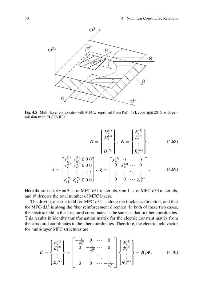
Fig. 4.5 Multi-layer composites with MFCs, reprinted from Ref. [18], copyright 2015, with permission from ELSEVIER
D =
⎧
⎪ ⎪ ⎪ ⎨
⎪ ⎪ ⎪ ⎩
D
(1)
s
D
(2)
s
. . .
D
(N )
s
⎫
⎪ ⎪ ⎪ ⎬
⎪ ⎪ ⎪ ⎭
, E =
⎧
⎪ ⎪ ⎪ ⎨
⎪ ⎪ ⎪ ⎩
E
(1)
s
E
(2)
s
. . .
E
(N )
s
⎫
⎪ ⎪ ⎪ ⎬
⎪ ⎪ ⎪ ⎭
,
(4.68)
e =
⎡
⎢
⎢
⎢
⎣
e
(1)
s1 e
(1)
s2 0 0 0
e
(2)
s1 e
(2)
s2 0 0 0
. . .
. . .
. . .
. . .
. . .
e
(N )
s1 e
(N )
s2 0 0 0
⎤
⎥
⎥
⎥
⎦
, χ =
⎡
⎢
⎢
⎢
⎣
χ
(1)
ss
0 · · · 0
0 χ
(2)
ss · · · 0
. . .
. . .
. . .
. . .
0 0 · · · χ
(N )
ss
⎤
⎥
⎥
⎥
⎦
.
(4.69)
Here the subscript s = 3 is for MFC-d31 materials, s = 1 is for MFC-d33 materials,
and N denotes the total number of MFC layers.
The driving electric field for MFC-d31 is along the thickness direction, and that
for MFC-d33 is along the fiber reinforcement direction. In both of these two cases,
the electric field in the structural coordinates is the same as that in fiber coordinates.
This results in identity transformation matrix for the electric constant matrix from
the structural coordinates to the fiber coordinates. Therefore, the electric field vector
for multi-layer MFC structures are
E =
⎧
⎪ ⎪ ⎪ ⎨
⎪ ⎪ ⎪ ⎩
E
(1)
s
E
(2)
s
. . .
E
(N )
s
⎫
⎪ ⎪ ⎪ ⎬
⎪ ⎪ ⎪ ⎭
=
⎡
⎢
⎢
⎢
⎢
⎢
⎣
−
1
h
(1)
E
0 · · · 0
0 −
1
h
(2)
E
· · · 0
. . .
. . .
. . .
. . .
0
0 · · · −
1
h
(N )
E
⎤
⎥
⎥
⎥
⎥
⎥
⎦
⎧
⎪ ⎪ ⎪ ⎨
⎪ ⎪ ⎪ ⎩
Φ
(1)
s
Φ
(2)
s
. . .
Φ
(N )
s
⎫
⎪ ⎪ ⎪ ⎬
⎪ ⎪ ⎪ ⎭
= B φ Φ,
(4.70)
4 Nonlinear Constitutive Relations
˘
Θ
1
˘
Θ
1
Θ
3
Θ
2
Θ
1
˘
Θ
1
F i b e r
˘
Θ
1
˘
Θ
2
θ
Fig. 4.5 Multi-layer composites with MFCs, reprinted from Ref. [18], copyright 2015, with permission from ELSEVIER
D =
⎧
⎪ ⎪ ⎪ ⎨
⎪ ⎪ ⎪ ⎩
D
(1)
s
D
(2)
s
. . .
D
(N )
s
⎫
⎪ ⎪ ⎪ ⎬
⎪ ⎪ ⎪ ⎭
, E =
⎧
⎪ ⎪ ⎪ ⎨
⎪ ⎪ ⎪ ⎩
E
(1)
s
E
(2)
s
. . .
E
(N )
s
⎫
⎪ ⎪ ⎪ ⎬
⎪ ⎪ ⎪ ⎭
,
(4.68)
e =
⎡
⎢
⎢
⎢
⎣
e
(1)
s1 e
(1)
s2 0 0 0
e
(2)
s1 e
(2)
s2 0 0 0
. . .
. . .
. . .
. . .
. . .
e
(N )
s1 e
(N )
s2 0 0 0
⎤
⎥
⎥
⎥
⎦
, χ =
⎡
⎢
⎢
⎢
⎣
χ
(1)
ss
0 · · · 0
0 χ
(2)
ss · · · 0
. . .
. . .
. . .
. . .
0 0 · · · χ
(N )
ss
⎤
⎥
⎥
⎥
⎦
.
(4.69)
Here the subscript s = 3 is for MFC-d31 materials, s = 1 is for MFC-d33 materials,
and N denotes the total number of MFC layers.
The driving electric field for MFC-d31 is along the thickness direction, and that
for MFC-d33 is along the fiber reinforcement direction. In both of these two cases,
the electric field in the structural coordinates is the same as that in fiber coordinates.
This results in identity transformation matrix for the electric constant matrix from
the structural coordinates to the fiber coordinates. Therefore, the electric field vector
for multi-layer MFC structures are
E =
⎧
⎪ ⎪ ⎪ ⎨
⎪ ⎪ ⎪ ⎩
E
(1)
s
E
(2)
s
. . .
E
(N )
s
⎫
⎪ ⎪ ⎪ ⎬
⎪ ⎪ ⎪ ⎭
=
⎡
⎢
⎢
⎢
⎢
⎢
⎣
−
1
h
(1)
E
0 · · · 0
0 −
1
h
(2)
E
· · · 0
. . .
. . .
. . .
. . .
0
0 · · · −
1
h
(N )
E
⎤
⎥
⎥
⎥
⎥
⎥
⎦
⎧
⎪ ⎪ ⎪ ⎨
⎪ ⎪ ⎪ ⎩
Φ
(1)
s
Φ
(2)
s
. . .
Φ
(N )
s
⎫
⎪ ⎪ ⎪ ⎬
⎪ ⎪ ⎪ ⎭
= B φ Φ,
(4.70)