

66
3 Continuum Mechanics and Nonlinear Elasticity
Solution
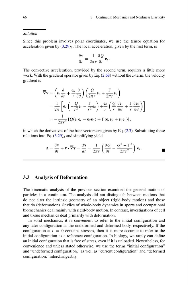
Since this problem involves polar coordinates, we use the tensor equation for
acceleration given by (3.29) 2 . The local acceleration, given by the first term, is
∂v
∂t
=
1
2πr
∂Q
∂t
e r .
The convective acceleration, provided by the second term, requires a little more
work. With the gradient operator given by Eq. (2.68) without the z-term, the velocity
gradient is
∇v =
e r
∂
∂r
+
e θ
r
∂
∂θ
Q
2πr
e r +
2πr
e θ
=
1
2π
e r
−
Q
r 2 e r −
r 2 e θ
+
e θ
r
Q
r
∂e r
∂θ
+
r
∂e θ
∂θ
= −
1
2πr 2 [Q(e r e r − e θ e θ ) + (e r e θ + e θ e r )] ,
in which the derivatives of the base vectors are given by Eq. (2.3). Substituting these
relations into Eq. (3.29) 2 and simplifying yield
a =
∂v
∂t
+ v · ∇v =
dv
dt
=
1
2πr
∂Q
∂t
−
Q 2 − 2
2πr 2
e r .
3.3 Analysis of Deformation
The kinematic analysis of the previous section examined the general motion of
particles in a continuum. The analysis did not distinguish between motions that
do not alter the intrinsic geometry of an object (rigid-body motion) and those
that do (deformation). Studies of whole-body dynamics in sports and occupational
biomechanics deal mainly with rigid-body motion. In contrast, investigations of cell
and tissue mechanics deal primarily with deformation.
In solid mechanics, it is convenient to refer to the initial configuration and
any later configuration as the undeformed and deformed body, respectively. If the
configuration at t = 0 contains stresses, then it is more accurate to refer to the
initial configuration as a reference configuration. In biology, we rarely can define
an initial configuration that is free of stress, even if it is unloaded. Nevertheless, for
convenience and unless stated otherwise, we use the terms “initial configuration”
and “undeformed configuration,” as well as “current configuration” and “deformed
configuration,” interchangeably.
3 Continuum Mechanics and Nonlinear Elasticity
Solution
Since this problem involves polar coordinates, we use the tensor equation for
acceleration given by (3.29) 2 . The local acceleration, given by the first term, is
∂v
∂t
=
1
2πr
∂Q
∂t
e r .
The convective acceleration, provided by the second term, requires a little more
work. With the gradient operator given by Eq. (2.68) without the z-term, the velocity
gradient is
∇v =
e r
∂
∂r
+
e θ
r
∂
∂θ
Q
2πr
e r +
2πr
e θ
=
1
2π
e r
−
Q
r 2 e r −
r 2 e θ
+
e θ
r
Q
r
∂e r
∂θ
+
r
∂e θ
∂θ
= −
1
2πr 2 [Q(e r e r − e θ e θ ) + (e r e θ + e θ e r )] ,
in which the derivatives of the base vectors are given by Eq. (2.3). Substituting these
relations into Eq. (3.29) 2 and simplifying yield
a =
∂v
∂t
+ v · ∇v =
dv
dt
=
1
2πr
∂Q
∂t
−
Q 2 − 2
2πr 2
e r .
3.3 Analysis of Deformation
The kinematic analysis of the previous section examined the general motion of
particles in a continuum. The analysis did not distinguish between motions that
do not alter the intrinsic geometry of an object (rigid-body motion) and those
that do (deformation). Studies of whole-body dynamics in sports and occupational
biomechanics deal mainly with rigid-body motion. In contrast, investigations of cell
and tissue mechanics deal primarily with deformation.
In solid mechanics, it is convenient to refer to the initial configuration and
any later configuration as the undeformed and deformed body, respectively. If the
configuration at t = 0 contains stresses, then it is more accurate to refer to the
initial configuration as a reference configuration. In biology, we rarely can define
an initial configuration that is free of stress, even if it is unloaded. Nevertheless, for
convenience and unless stated otherwise, we use the terms “initial configuration”
and “undeformed configuration,” as well as “current configuration” and “deformed
configuration,” interchangeably.