

524
B Fourier Series
a 0 =
1
2L
L
−L
f (x) dx
a n =
1
L
L
−L
f (x) cos
nπ x
L
dx, n = 1, 2, . . .
b n =
1
L
L
−L
f (x) sin
nπ x
L
dx, n = 1, 2, . . . .
(B.3)
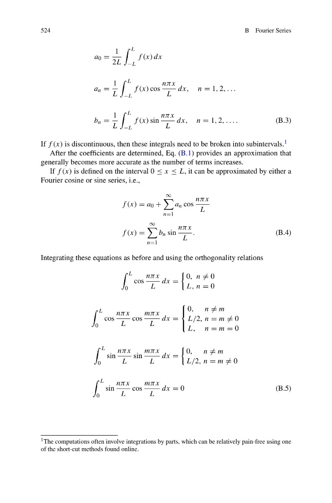
If f (x) is discontinuous, then these integrals need to be broken into subintervals. 1
After the coefficients are determined, Eq. (B.1) provides an approximation that
generally becomes more accurate as the number of terms increases.
If f (x) is defined on the interval 0 ≤ x ≤ L, it can be approximated by either a
Fourier cosine or sine series, i.e.,
f (x) = a 0 +
∞
n=1
a n cos
nπ x
L
f (x) =
∞
n=1
b n sin
nπ x
L
.
(B.4)
Integrating these equations as before and using the orthogonality relations
L
0
cos
nπ x
L
dx =
0, n = 0
L, n = 0
L
0
cos
nπ x
L
cos
mπ x
L
dx =
⎧
⎨
⎩
0, n = m
L/2, n = m = 0
L, n = m = 0
L
0
sin
nπ x
L
sin
mπx
L
dx =
0, n = m
L/2, n = m = 0
L
0
sin
nπ x
L
cos
mπ x
L
dx = 0
( B . 5 )
1 The computations often involve integrations by parts, which can be relatively pain-free using one
of the short-cut methods found online.
B Fourier Series
a 0 =
1
2L
L
−L
f (x) dx
a n =
1
L
L
−L
f (x) cos
nπ x
L
dx, n = 1, 2, . . .
b n =
1
L
L
−L
f (x) sin
nπ x
L
dx, n = 1, 2, . . . .
(B.3)
If f (x) is discontinuous, then these integrals need to be broken into subintervals. 1
After the coefficients are determined, Eq. (B.1) provides an approximation that
generally becomes more accurate as the number of terms increases.
If f (x) is defined on the interval 0 ≤ x ≤ L, it can be approximated by either a
Fourier cosine or sine series, i.e.,
f (x) = a 0 +
∞
n=1
a n cos
nπ x
L
f (x) =
∞
n=1
b n sin
nπ x
L
.
(B.4)
Integrating these equations as before and using the orthogonality relations
L
0
cos
nπ x
L
dx =
0, n = 0
L, n = 0
L
0
cos
nπ x
L
cos
mπ x
L
dx =
⎧
⎨
⎩
0, n = m
L/2, n = m = 0
L, n = m = 0
L
0
sin
nπ x
L
sin
mπx
L
dx =
0, n = m
L/2, n = m = 0
L
0
sin
nπ x
L
cos
mπ x
L
dx = 0
( B . 5 )
1 The computations often involve integrations by parts, which can be relatively pain-free using one
of the short-cut methods found online.