

Appendix B
Fourier Series
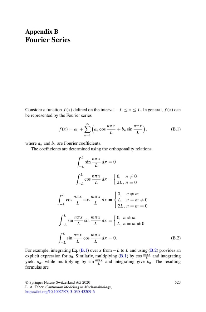
Consider a function f (x) defined on the interval −L ≤ x ≤ L. In general, f (x) can
be represented by the Fourier series
f (x) = a 0 +
∞
n=1
a n cos
nπ x
L
+ b n sin
nπ x
L
,
(B.1)
where a n and b n are Fourier coefficients.
The coefficients are determined using the orthogonality relations
L
−L
sin
nπ x
L
dx = 0
L
−L
cos
nπ x
L
dx =
0, n = 0
2L, n = 0
L
−L
cos
nπ x
L
cos
mπ x
L
dx =
⎧
⎨
⎩
0, n = m
L, n = m = 0
2L, n = m = 0
L
−L
sin
nπ x
L
sin
mπx
L
dx =
0, n = m
L, n = m = 0
L
−L
sin
nπ x
L
cos
mπ x
L
dx = 0.
(B.2)
For example, integrating Eq. (B.1) over x from −L to L and using (B.2) provides an
explicit expression for a 0 . Similarly, multiplying (B.1) by cos
mπ x
L and integrating
yield a n , while multiplying by sin
mπ x
L and integrating give b n . The resulting
formulas are
© Springer Nature Switzerland AG 2020
L. A. Taber, Continuum Modeling in Mechanobiology,
https://doi.org/10.1007/978-3-030-43209-6
523
Fourier Series
Consider a function f (x) defined on the interval −L ≤ x ≤ L. In general, f (x) can
be represented by the Fourier series
f (x) = a 0 +
∞
n=1
a n cos
nπ x
L
+ b n sin
nπ x
L
,
(B.1)
where a n and b n are Fourier coefficients.
The coefficients are determined using the orthogonality relations
L
−L
sin
nπ x
L
dx = 0
L
−L
cos
nπ x
L
dx =
0, n = 0
2L, n = 0
L
−L
cos
nπ x
L
cos
mπ x
L
dx =
⎧
⎨
⎩
0, n = m
L, n = m = 0
2L, n = m = 0
L
−L
sin
nπ x
L
sin
mπx
L
dx =
0, n = m
L, n = m = 0
L
−L
sin
nπ x
L
cos
mπ x
L
dx = 0.
(B.2)
For example, integrating Eq. (B.1) over x from −L to L and using (B.2) provides an
explicit expression for a 0 . Similarly, multiplying (B.1) by cos
mπ x
L and integrating
yield a n , while multiplying by sin
mπ x
L and integrating give b n . The resulting
formulas are
© Springer Nature Switzerland AG 2020
L. A. Taber, Continuum Modeling in Mechanobiology,
https://doi.org/10.1007/978-3-030-43209-6
523