

7.6 Case Study: Growth and Remodeling of Arteries
375
Solution Procedure After defining a grid across the wall at t = 0, we use the
initial conditions (7.76) and step forward in time. The computational procedure at
each time step is the following:
1. Compute P and Q using (6.121).
2. With λ given, solve (7.84) 2 for a. 4 Each iteration requires the following steps:
(a) Compute r, λ i , λ m∗
i , and λ n∗
θ at each R using (7.82), (7.73), and (7.74),
respectively.
(b) Compute ¯
σ i (σ i excluding p) at each R using (7.71), (7.78), and (7.79).
3. Integrate (7.84) 1 to obtain p(R) and compute σ i = ¯
σ i − p.
4. Compute τ f from (7.81).
5. For P = 0, compute residual stresses and opening angles using the procedure
described in Sect. 6.11.4.
6. For each R, integrate (7.72) to obtain G m
i for the next time step, and so on.
Illustrative Results In the following, time t = 0 is shifted to correspond to the
time in the mature artery when the blood pressure begins to build toward a 50%
increase. All plotted results pertain to the time period t ≥ 0.
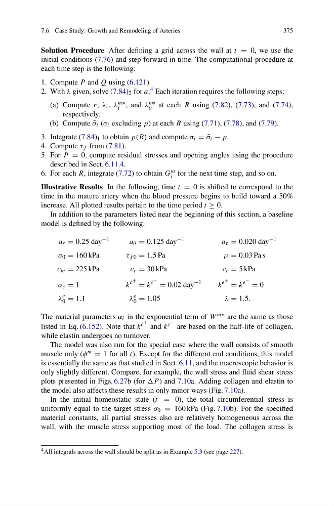
In addition to the parameters listed near the beginning of this section, a baseline
model is defined by the following:
a r = 0.25 day
−1
a θ = 0.125 day
−1
a τ = 0.020 day
−1
σ 0 = 160 kPa
τ f 0 = 1.5 Pa
μ = 0.03 Pa s
c m = 225 kPa
c c = 30 kPa
c e = 5 kPa
α c = 1
k
c + = k
c − = 0.02 day
−1
k
e + = k
e − = 0
λ
c
0 = 1.1
λ
e
0 = 1.05
λ = 1.5.
The material parameters α i in the exponential term of W m∗ are the same as those
listed in Eq. (6.152). Note that k c + and k c − are based on the half-life of collagen,
while elastin undergoes no turnover.
The model was also run for the special case where the wall consists of smooth
muscle only (φ m = 1 for all t). Except for the different end conditions, this model
is essentially the same as that studied in Sect. 6.11, and the macroscopic behavior is
only slightly different. Compare, for example, the wall stress and fluid shear stress
plots presented in Figs. 6.27b (for P ) and 7.10a. Adding collagen and elastin to
the model also affects these results in only minor ways (Fig. 7.10a).
In the initial homeostatic state (t = 0), the total circumferential stress is
uniformly equal to the target stress σ 0 = 160 kPa (Fig. 7.10b). For the specified
material constants, all partial stresses also are relatively homogeneous across the
wall, with the muscle stress supporting most of the load. The collagen stress is
4 All integrals across the wall should be split as in Example 5.3 (see page 227).
375
Solution Procedure After defining a grid across the wall at t = 0, we use the
initial conditions (7.76) and step forward in time. The computational procedure at
each time step is the following:
1. Compute P and Q using (6.121).
2. With λ given, solve (7.84) 2 for a. 4 Each iteration requires the following steps:
(a) Compute r, λ i , λ m∗
i , and λ n∗
θ at each R using (7.82), (7.73), and (7.74),
respectively.
(b) Compute ¯
σ i (σ i excluding p) at each R using (7.71), (7.78), and (7.79).
3. Integrate (7.84) 1 to obtain p(R) and compute σ i = ¯
σ i − p.
4. Compute τ f from (7.81).
5. For P = 0, compute residual stresses and opening angles using the procedure
described in Sect. 6.11.4.
6. For each R, integrate (7.72) to obtain G m
i for the next time step, and so on.
Illustrative Results In the following, time t = 0 is shifted to correspond to the
time in the mature artery when the blood pressure begins to build toward a 50%
increase. All plotted results pertain to the time period t ≥ 0.
In addition to the parameters listed near the beginning of this section, a baseline
model is defined by the following:
a r = 0.25 day
−1
a θ = 0.125 day
−1
a τ = 0.020 day
−1
σ 0 = 160 kPa
τ f 0 = 1.5 Pa
μ = 0.03 Pa s
c m = 225 kPa
c c = 30 kPa
c e = 5 kPa
α c = 1
k
c + = k
c − = 0.02 day
−1
k
e + = k
e − = 0
λ
c
0 = 1.1
λ
e
0 = 1.05
λ = 1.5.
The material parameters α i in the exponential term of W m∗ are the same as those
listed in Eq. (6.152). Note that k c + and k c − are based on the half-life of collagen,
while elastin undergoes no turnover.
The model was also run for the special case where the wall consists of smooth
muscle only (φ m = 1 for all t). Except for the different end conditions, this model
is essentially the same as that studied in Sect. 6.11, and the macroscopic behavior is
only slightly different. Compare, for example, the wall stress and fluid shear stress
plots presented in Figs. 6.27b (for P ) and 7.10a. Adding collagen and elastin to
the model also affects these results in only minor ways (Fig. 7.10a).
In the initial homeostatic state (t = 0), the total circumferential stress is
uniformly equal to the target stress σ 0 = 160 kPa (Fig. 7.10b). For the specified
material constants, all partial stresses also are relatively homogeneous across the
wall, with the muscle stress supporting most of the load. The collagen stress is
4 All integrals across the wall should be split as in Example 5.3 (see page 227).