

7.5 General Theory for Growth and Remodeling in 3D
367
as the initial conditions for the growth of each constituent. Finally, Eq. (7.6) 1
provides
J = J
κ
+
N
n=1
J
n .
(7.56)
For the fibers, Eq. (7.13) provides the partial volume ratio
J
n (t) = J
n (0)q
n (t, 0) +
t
0
˙
J
n + (τ )q
n (t, τ ) dτ.
(7.57)
From this relation, fiber growth ratios can be computed using J n = G n
1 G n
2 G n
3 and
assumptions like those used to define anisotropic growth in Eqs. (7.23) and (7.24).
For the cells, as before, G κ can be a specified function of time or determined using
growth laws; then J κ = det G κ .
7.5.2 Kinematics
With contraction ignored, the various configurations for the cells are the same as
those depicted in Fig. 6.10, which shows the pathway linking the initial and current
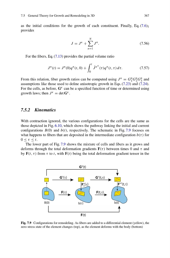
configurations B(0) and b(t), respectively. The schematic in Fig. 7.9 focuses on
what happens to fibers that are deposited in the intermediate configuration b(τ ) for
0 ≤ τ ≤ t.
The lower part of Fig. 7.9 shows the mixture of cells and fibers as it grows and
deforms through the total deformation gradients F(τ ) between times 0 and τ and
by F(t, τ ) from τ to t, with F(t) being the total deformation gradient tensor in the
)
t
(
b
)
0
(
B
F(W)
F(t)
b(W)
F(t,W)
G
n
(W)
G
n
(t,W)
F
n*
(t,W)
G
n
(t)
F 0
n
(W)
Fig. 7.9 Configurations for remodeling. As fibers are added to a differential element (yellow), the
zero-stress state of the element changes (top), as the element deforms with the body (bottom)
367
as the initial conditions for the growth of each constituent. Finally, Eq. (7.6) 1
provides
J = J
κ
+
N
n=1
J
n .
(7.56)
For the fibers, Eq. (7.13) provides the partial volume ratio
J
n (t) = J
n (0)q
n (t, 0) +
t
0
˙
J
n + (τ )q
n (t, τ ) dτ.
(7.57)
From this relation, fiber growth ratios can be computed using J n = G n
1 G n
2 G n
3 and
assumptions like those used to define anisotropic growth in Eqs. (7.23) and (7.24).
For the cells, as before, G κ can be a specified function of time or determined using
growth laws; then J κ = det G κ .
7.5.2 Kinematics
With contraction ignored, the various configurations for the cells are the same as
those depicted in Fig. 6.10, which shows the pathway linking the initial and current
configurations B(0) and b(t), respectively. The schematic in Fig. 7.9 focuses on
what happens to fibers that are deposited in the intermediate configuration b(τ ) for
0 ≤ τ ≤ t.
The lower part of Fig. 7.9 shows the mixture of cells and fibers as it grows and
deforms through the total deformation gradients F(τ ) between times 0 and τ and
by F(t, τ ) from τ to t, with F(t) being the total deformation gradient tensor in the
)
t
(
b
)
0
(
B
F(W)
F(t)
b(W)
F(t,W)
G
n
(W)
G
n
(t,W)
F
n*
(t,W)
G
n
(t)
F 0
n
(W)
Fig. 7.9 Configurations for remodeling. As fibers are added to a differential element (yellow), the
zero-stress state of the element changes (top), as the element deforms with the body (bottom)