

170
4 Problems in Soft Tissue Biomechanics
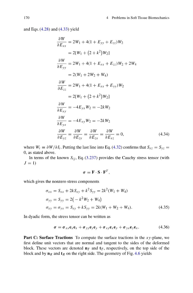
and Eqs. (4.28) and (4.33) yield
∂W
∂E xx
= 2W 1 + 4(1 + E yy + E zz )W 2
= 2[W 1 +
2 + k
2
W 2 ]
∂W
∂E yy
= 2W 1 + 4(1 + E xx + E zz )W 2 + 2W 4
= 2(W 1 + 2W 2 + W 4 )
∂W
∂E zz
= 2W 1 + 4(1 + E xx + E yy )W 2
= 2[W 1 +
2 + k
2
W 2 ]
∂W
∂E xy
= −4E yx W 2 = −2kW 2
∂W
∂E yx
= −4E xy W 2 = −2kW 2
∂W
∂E yz
=
∂W
∂E zy
=
∂W
∂E zx
=
∂W
∂E xz
= 0,
(4.34)
where W i ≡ ∂W/∂I i . Putting the last line into Eq. (4.32) confirms that S xz = S yz =
0, as stated above.
In terms of the known S ij , Eq. (3.237) provides the Cauchy stress tensor (with
J = 1)
σ = F · S · F
T ,
which gives the nonzero stress components
σ xx = S xx + 2kS xy + k
2 S yy = 2k
2 (W 1 + W 4 )
σ yy = S yy = 2
− k
2 W 2 + W 4
σ xy = σ yx = S xy + kS yy = 2k(W 1 + W 2 + W 4 ).
(4.35)
In dyadic form, the stress tensor can be written as
σ = σ xx e x e x + σ yy e y e y + σ xy e x e y + σ yx e y e x .
(4.36)
Part C: Surface Tractions To compute the surface tractions in the xy-plane, we
first define unit vectors that are normal and tangent to the sides of the deformed
block. These vectors are denoted n T and t T , respectively, on the top side of the
block and by n R and t R on the right side. The geometry of Fig. 4.6 yields
4 Problems in Soft Tissue Biomechanics
and Eqs. (4.28) and (4.33) yield
∂W
∂E xx
= 2W 1 + 4(1 + E yy + E zz )W 2
= 2[W 1 +
2 + k
2
W 2 ]
∂W
∂E yy
= 2W 1 + 4(1 + E xx + E zz )W 2 + 2W 4
= 2(W 1 + 2W 2 + W 4 )
∂W
∂E zz
= 2W 1 + 4(1 + E xx + E yy )W 2
= 2[W 1 +
2 + k
2
W 2 ]
∂W
∂E xy
= −4E yx W 2 = −2kW 2
∂W
∂E yx
= −4E xy W 2 = −2kW 2
∂W
∂E yz
=
∂W
∂E zy
=
∂W
∂E zx
=
∂W
∂E xz
= 0,
(4.34)
where W i ≡ ∂W/∂I i . Putting the last line into Eq. (4.32) confirms that S xz = S yz =
0, as stated above.
In terms of the known S ij , Eq. (3.237) provides the Cauchy stress tensor (with
J = 1)
σ = F · S · F
T ,
which gives the nonzero stress components
σ xx = S xx + 2kS xy + k
2 S yy = 2k
2 (W 1 + W 4 )
σ yy = S yy = 2
− k
2 W 2 + W 4
σ xy = σ yx = S xy + kS yy = 2k(W 1 + W 2 + W 4 ).
(4.35)
In dyadic form, the stress tensor can be written as
σ = σ xx e x e x + σ yy e y e y + σ xy e x e y + σ yx e y e x .
(4.36)
Part C: Surface Tractions To compute the surface tractions in the xy-plane, we
first define unit vectors that are normal and tangent to the sides of the deformed
block. These vectors are denoted n T and t T , respectively, on the top side of the
block and by n R and t R on the right side. The geometry of Fig. 4.6 yields