

4.3 Shear of a Block
167
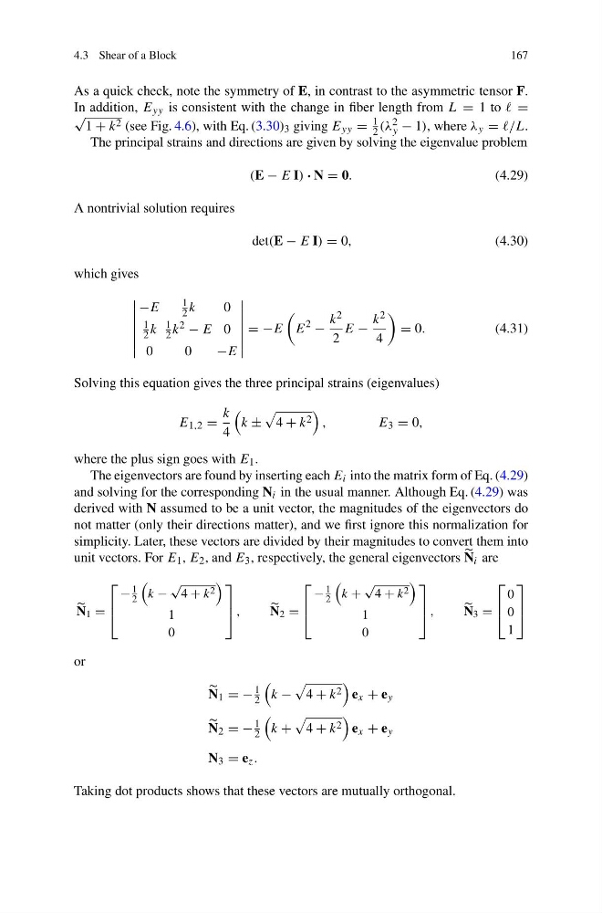
As a quick check, note the symmetry of E, in contrast to the asymmetric tensor F.
In addition, E yy is consistent with the change in fiber length from L = 1 to =
√
1 + k 2 (see Fig. 4.6), with Eq. (3.30) 3 giving E yy =
1
2 (λ 2
y − 1), where λ y = /L.
The principal strains and directions are given by solving the eigenvalue problem
(E − E I) · N = 0.
(4.29)
A nontrivial solution requires
det(E − E I) = 0,
(4.30)
which gives
−E
1
2 k
0
1
2 k
1
2 k 2 − E 0
0
0
−E
= −E
E
2
−
k 2
2
E −
k 2
4
= 0.
(4.31)
Solving this equation gives the three principal strains (eigenvalues)
E 1,2 =
k
4
k ±
4 + k 2
,
E 3 = 0,
where the plus sign goes with E 1 .
The eigenvectors are found by inserting each E i into the matrix form of Eq. (4.29)
and solving for the corresponding N i in the usual manner. Although Eq. (4.29) was
derived with N assumed to be a unit vector, the magnitudes of the eigenvectors do
not matter (only their directions matter), and we first ignore this normalization for
simplicity. Later, these vectors are divided by their magnitudes to convert them into
unit vectors. For E 1 , E 2 , and E 3 , respectively, the general eigenvectors N i are
N 1 =
⎡
⎢
⎣
−
1
2
k −
√
4 + k 2
1
0
⎤
⎥
⎦ ,
N 2 =
⎡
⎢
⎣
−
1
2
k +
√
4 + k 2
1
0
⎤
⎥
⎦ ,
N 3 =
⎡
⎢
⎣
0
0
1
⎤
⎥
⎦
or
N 1 = −
1
2
k −
4 + k 2
e x + e y
N 2 = −
1
2
k +
4 + k 2
e x + e y
N 3 = e z .
Taking dot products shows that these vectors are mutually orthogonal.
167
As a quick check, note the symmetry of E, in contrast to the asymmetric tensor F.
In addition, E yy is consistent with the change in fiber length from L = 1 to =
√
1 + k 2 (see Fig. 4.6), with Eq. (3.30) 3 giving E yy =
1
2 (λ 2
y − 1), where λ y = /L.
The principal strains and directions are given by solving the eigenvalue problem
(E − E I) · N = 0.
(4.29)
A nontrivial solution requires
det(E − E I) = 0,
(4.30)
which gives
−E
1
2 k
0
1
2 k
1
2 k 2 − E 0
0
0
−E
= −E
E
2
−
k 2
2
E −
k 2
4
= 0.
(4.31)
Solving this equation gives the three principal strains (eigenvalues)
E 1,2 =
k
4
k ±
4 + k 2
,
E 3 = 0,
where the plus sign goes with E 1 .
The eigenvectors are found by inserting each E i into the matrix form of Eq. (4.29)
and solving for the corresponding N i in the usual manner. Although Eq. (4.29) was
derived with N assumed to be a unit vector, the magnitudes of the eigenvectors do
not matter (only their directions matter), and we first ignore this normalization for
simplicity. Later, these vectors are divided by their magnitudes to convert them into
unit vectors. For E 1 , E 2 , and E 3 , respectively, the general eigenvectors N i are
N 1 =
⎡
⎢
⎣
−
1
2
k −
√
4 + k 2
1
0
⎤
⎥
⎦ ,
N 2 =
⎡
⎢
⎣
−
1
2
k +
√
4 + k 2
1
0
⎤
⎥
⎦ ,
N 3 =
⎡
⎢
⎣
0
0
1
⎤
⎥
⎦
or
N 1 = −
1
2
k −
4 + k 2
e x + e y
N 2 = −
1
2
k +
4 + k 2
e x + e y
N 3 = e z .
Taking dot products shows that these vectors are mutually orthogonal.