

134
3 Continuum Mechanics and Nonlinear Elasticity
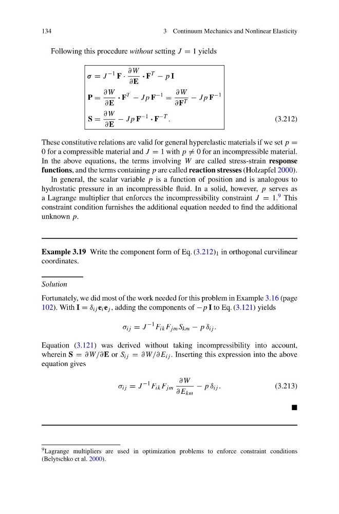
Following this procedure without setting J = 1 yields
σ = J
−1 F ·
∂W
∂E
· F
T
− p I
P =
∂W
∂E
· F
T
− Jp F
−1
=
∂W
∂F T − Jp F
−1
S =
∂W
∂E
− Jp F
−1
· F
−T .
(3.212)
These constitutive relations are valid for general hyperelastic materials if we set p =
0 for a compressible material and J = 1 with p = 0 for an incompressible material.
In the above equations, the terms involving W are called stress-strain response
functions, and the terms containing p are called reaction stresses (Holzapfel 2000).
In general, the scalar variable p is a function of position and is analogous to
hydrostatic pressure in an incompressible fluid. In a solid, however, p serves as
a Lagrange multiplier that enforces the incompressibility constraint J = 1. 9 This
constraint condition furnishes the additional equation needed to find the additional
unknown p.
Example 3.19 Write the component form of Eq. (3.212) 1 in orthogonal curvilinear
coordinates.
Solution
Fortunately, we did most of the work needed for this problem in Example 3.16 (page
102). With I = δ ij e i e j , adding the components of −p I to Eq. (3.121) yields
σ ij = J
−1 F ik F jm S km − p δ ij .
Equation (3.121) was derived without taking incompressibility into account,
wherein S = ∂W/∂E or S ij = ∂W/∂E ij . Inserting this expression into the above
equation gives
σ ij = J
−1 F ik F jm
∂W
∂E km
− p δ ij .
(3.213)
9 Lagrange multipliers are used in optimization problems to enforce constraint conditions
(Belytschko et al. 2000).
3 Continuum Mechanics and Nonlinear Elasticity
Following this procedure without setting J = 1 yields
σ = J
−1 F ·
∂W
∂E
· F
T
− p I
P =
∂W
∂E
· F
T
− Jp F
−1
=
∂W
∂F T − Jp F
−1
S =
∂W
∂E
− Jp F
−1
· F
−T .
(3.212)
These constitutive relations are valid for general hyperelastic materials if we set p =
0 for a compressible material and J = 1 with p = 0 for an incompressible material.
In the above equations, the terms involving W are called stress-strain response
functions, and the terms containing p are called reaction stresses (Holzapfel 2000).
In general, the scalar variable p is a function of position and is analogous to
hydrostatic pressure in an incompressible fluid. In a solid, however, p serves as
a Lagrange multiplier that enforces the incompressibility constraint J = 1. 9 This
constraint condition furnishes the additional equation needed to find the additional
unknown p.
Example 3.19 Write the component form of Eq. (3.212) 1 in orthogonal curvilinear
coordinates.
Solution
Fortunately, we did most of the work needed for this problem in Example 3.16 (page
102). With I = δ ij e i e j , adding the components of −p I to Eq. (3.121) yields
σ ij = J
−1 F ik F jm S km − p δ ij .
Equation (3.121) was derived without taking incompressibility into account,
wherein S = ∂W/∂E or S ij = ∂W/∂E ij . Inserting this expression into the above
equation gives
σ ij = J
−1 F ik F jm
∂W
∂E km
− p δ ij .
(3.213)
9 Lagrange multipliers are used in optimization problems to enforce constraint conditions
(Belytschko et al. 2000).