

3.4 Analysis of Stress
95
F
B
b
B 1
B 2
b
b 1
b 2
df df
~
df
T
0
~
T
M
N
T
m
n
(a)
(b)
(c)
F
dA
0
dA
dA
Y
X
dA
0
-1
y
x
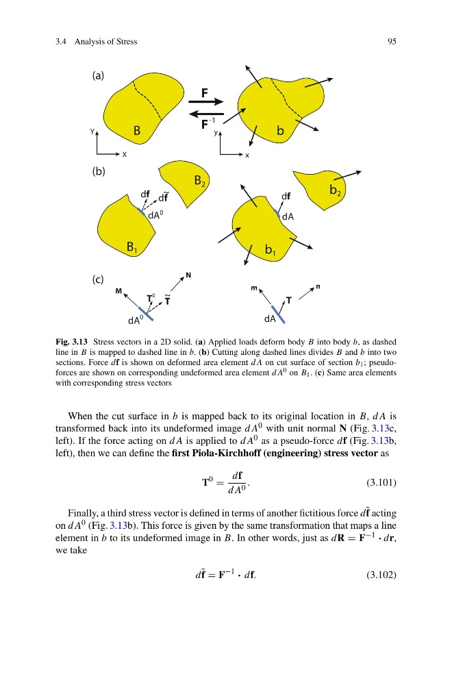
Fig. 3.13 Stress vectors in a 2D solid. (a) Applied loads deform body B into body b, as dashed
line in B is mapped to dashed line in b. (b) Cutting along dashed lines divides B and b into two
sections. Force df is shown on deformed area element dA on cut surface of section b 1 ; pseudoforces are shown on corresponding undeformed area element dA 0 on B 1 . (c) Same area elements
with corresponding stress vectors
When the cut surface in b is mapped back to its original location in B, dA is
transformed back into its undeformed image dA 0 with unit normal N (Fig. 3.13c,
left). If the force acting on dA is applied to dA 0 as a pseudo-force df (Fig. 3.13b,
left), then we can define the first Piola-Kirchhoff (engineering) stress vector as
T
0
=
df
dA 0 .
(3.101)
Finally, a third stress vector is defined in terms of another fictitious force d ˜ f acting
on dA 0 (Fig. 3.13b). This force is given by the same transformation that maps a line
element in b to its undeformed image in B. In other words, just as dR = F −1 · dr,
we take
d ˜ f = F
−1
· df.
(3.102)
95
F
B
b
B 1
B 2
b
b 1
b 2
df df
~
df
T
0
~
T
M
N
T
m
n
(a)
(b)
(c)
F
dA
0
dA
dA
Y
X
dA
0
-1
y
x
Fig. 3.13 Stress vectors in a 2D solid. (a) Applied loads deform body B into body b, as dashed
line in B is mapped to dashed line in b. (b) Cutting along dashed lines divides B and b into two
sections. Force df is shown on deformed area element dA on cut surface of section b 1 ; pseudoforces are shown on corresponding undeformed area element dA 0 on B 1 . (c) Same area elements
with corresponding stress vectors
When the cut surface in b is mapped back to its original location in B, dA is
transformed back into its undeformed image dA 0 with unit normal N (Fig. 3.13c,
left). If the force acting on dA is applied to dA 0 as a pseudo-force df (Fig. 3.13b,
left), then we can define the first Piola-Kirchhoff (engineering) stress vector as
T
0
=
df
dA 0 .
(3.101)
Finally, a third stress vector is defined in terms of another fictitious force d ˜ f acting
on dA 0 (Fig. 3.13b). This force is given by the same transformation that maps a line
element in b to its undeformed image in B. In other words, just as dR = F −1 · dr,
we take
d ˜ f = F
−1
· df.
(3.102)