

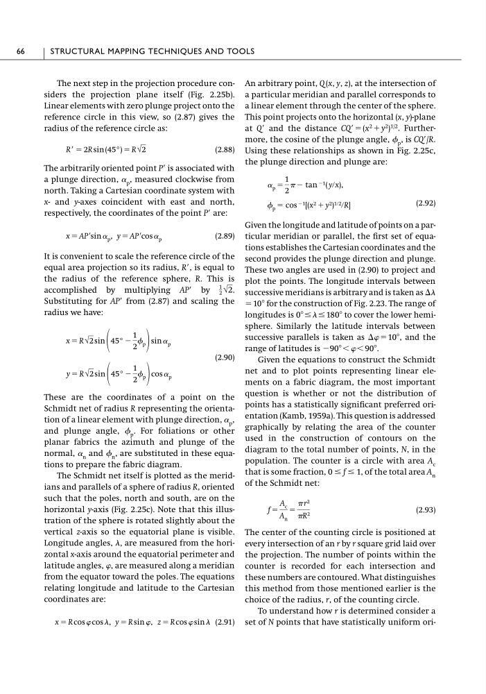
The next step in the projection procedure considers the projection plane itself (Fig. 2.25b).
Linear elements with zero plunge project onto the
reference circle in this view, so (2.87) gives the
radius of the reference circle as:
(2.88)
The arbitrarily oriented point P� is associated with
a plunge direction, � p , measured clockwise from
north. Taking a Cartesian coordinate system with
x- and y-axes coincident with east and north,
respectively, the coordinates of the point P� are:
(2.89)
It is convenient to scale the reference circle of the
equal area projection so its radius, R�, is equal to
the radius of the reference sphere, R. This is
accomplished by multiplying AP� by
.
Substituting for AP� from (2.87) and scaling the
radius we have:
(2.90)
These are the coordinates of a point on the
Schmidt net of radius R representing the orientation of a linear element with plunge direction, � p ,
and plunge angle, � p . For foliations or other
planar fabrics the azimuth and plunge of the
normal, � n and � n , are substituted in these equations to prepare the fabric diagram.
The Schmidt net itself is plotted as the meridians and parallels of a sphere of radius R, oriented
such that the poles, north and south, are on the
horizontal y-axis (Fig. 2.25c). Note that this illustration of the sphere is rotated slightly about the
vertical z-axis so the equatorial plane is visible.
Longitude angles, �, are measured from the horizontal x-axis around the equatorial perimeter and
latitude angles, �, are measured along a meridian
from the equator toward the poles. The equations
relating longitude and latitude to the Cartesian
coordinates are:
(2.91)
z � R cos � sin �
x � R cos � cos �, y � R sin �,
y � R √2 sin 45° �
1
2
� p cos � p
x � R √2 sin
45° �
1
2
� p
sin � p
1
2 √2
x � AP� sin � p , y � AP� cos � p
R� � 2R sin (45°) � R √2
An arbitrary point, Q (x, y, z), at the intersection of
a particular meridian and parallel corresponds to
a linear element through the center of the sphere.
This point projects onto the horizontal (x, y)-plane
at Q� and the distance CQ��(x
2 � y
2 )
1/2 . Furthermore, the cosine of the plunge angle, � p , is CQ�/R.
Using these relationships as shown in Fig. 2.25c,
the plunge direction and plunge are:
(2.92)
Given the longitude and latitude of points on a particular meridian or parallel, the first set of equations establishes the Cartesian coordinates and the
second provides the plunge direction and plunge.
These two angles are used in (2.90) to project and
plot the points. The longitude intervals between
successive meridians is arbitrary and is taken as ��
� 10� for the construction of Fig. 2.23. The range of
longitudes is 0��� � 180� to cover the lower hemisphere. Similarly the latitude intervals between
successive parallels is taken as �� � 10�, and the
range of latitudes is �90��� � 90�.
Given the equations to construct the Schmidt
net and to plot points representing linear elements on a fabric diagram, the most important
question is whether or not the distribution of
points has a statistically significant preferred orientation (Kamb, 1959a). This question is addressed
graphically by relating the area of the counter
used in the construction of contours on the
diagram to the total number of points, N, in the
population. The counter is a circle with area A c
that is some fraction, 0 � f � 1, of the total area A n
of the Schmidt net:
(2.93)
The center of the counting circle is positioned at
every intersection of an r by r square grid laid over
the projection. The number of points within the
counter is recorded for each intersection and
these numbers are contoured. What distinguishes
this method from those mentioned earlier is the
choice of the radius, r, of the counting circle.
To understand how r is determined consider a
set of N points that have statistically uniform orif �
A c
A n
�
� r 2
�R 2
� p � cos �1 [(x 2 � y 2 ) 1�2 �R]
� p �
1
2
� � tan �1 ( y�x),
66
STRUCTURAL MAPPING TECHNIQUES AND TOOLS
Linear elements with zero plunge project onto the
reference circle in this view, so (2.87) gives the
radius of the reference circle as:
(2.88)
The arbitrarily oriented point P� is associated with
a plunge direction, � p , measured clockwise from
north. Taking a Cartesian coordinate system with
x- and y-axes coincident with east and north,
respectively, the coordinates of the point P� are:
(2.89)
It is convenient to scale the reference circle of the
equal area projection so its radius, R�, is equal to
the radius of the reference sphere, R. This is
accomplished by multiplying AP� by
.
Substituting for AP� from (2.87) and scaling the
radius we have:
(2.90)
These are the coordinates of a point on the
Schmidt net of radius R representing the orientation of a linear element with plunge direction, � p ,
and plunge angle, � p . For foliations or other
planar fabrics the azimuth and plunge of the
normal, � n and � n , are substituted in these equations to prepare the fabric diagram.
The Schmidt net itself is plotted as the meridians and parallels of a sphere of radius R, oriented
such that the poles, north and south, are on the
horizontal y-axis (Fig. 2.25c). Note that this illustration of the sphere is rotated slightly about the
vertical z-axis so the equatorial plane is visible.
Longitude angles, �, are measured from the horizontal x-axis around the equatorial perimeter and
latitude angles, �, are measured along a meridian
from the equator toward the poles. The equations
relating longitude and latitude to the Cartesian
coordinates are:
(2.91)
z � R cos � sin �
x � R cos � cos �, y � R sin �,
y � R √2 sin 45° �
1
2
� p cos � p
x � R √2 sin
45° �
1
2
� p
sin � p
1
2 √2
x � AP� sin � p , y � AP� cos � p
R� � 2R sin (45°) � R √2
An arbitrary point, Q (x, y, z), at the intersection of
a particular meridian and parallel corresponds to
a linear element through the center of the sphere.
This point projects onto the horizontal (x, y)-plane
at Q� and the distance CQ��(x
2 � y
2 )
1/2 . Furthermore, the cosine of the plunge angle, � p , is CQ�/R.
Using these relationships as shown in Fig. 2.25c,
the plunge direction and plunge are:
(2.92)
Given the longitude and latitude of points on a particular meridian or parallel, the first set of equations establishes the Cartesian coordinates and the
second provides the plunge direction and plunge.
These two angles are used in (2.90) to project and
plot the points. The longitude intervals between
successive meridians is arbitrary and is taken as ��
� 10� for the construction of Fig. 2.23. The range of
longitudes is 0��� � 180� to cover the lower hemisphere. Similarly the latitude intervals between
successive parallels is taken as �� � 10�, and the
range of latitudes is �90��� � 90�.
Given the equations to construct the Schmidt
net and to plot points representing linear elements on a fabric diagram, the most important
question is whether or not the distribution of
points has a statistically significant preferred orientation (Kamb, 1959a). This question is addressed
graphically by relating the area of the counter
used in the construction of contours on the
diagram to the total number of points, N, in the
population. The counter is a circle with area A c
that is some fraction, 0 � f � 1, of the total area A n
of the Schmidt net:
(2.93)
The center of the counting circle is positioned at
every intersection of an r by r square grid laid over
the projection. The number of points within the
counter is recorded for each intersection and
these numbers are contoured. What distinguishes
this method from those mentioned earlier is the
choice of the radius, r, of the counting circle.
To understand how r is determined consider a
set of N points that have statistically uniform orif �
A c
A n
�
� r 2
�R 2
� p � cos �1 [(x 2 � y 2 ) 1�2 �R]
� p �
1
2
� � tan �1 ( y�x),
66
STRUCTURAL MAPPING TECHNIQUES AND TOOLS