

new coordinates, P(xЈ, yЈ), which are found using
the following equations:
(2.13)
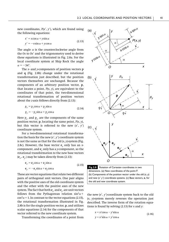
The angle ␣ is the counterclockwise angle from
the Ox to OxЈ and the trigonometry used to derive
these equations is illustrated in Fig. 2.8a. For the
local coordinate system at Ship Rock the angle
␣ ϭϪ34Њ.
The x- and y-components of position vectors p
and q (Fig. 2.8b) change under the rotational
transformation just described, but the position
vectors themselves are unchanged. Because the
components of an arbitrary position vector, p,
that locates a point, P(x, y), are equivalent to the
coordinates of that point, the two-dimensional
rotational transformation of position vectors
about the z-axis follows directly from (2.13):
(2.14)
Here p xЈ and p yЈ are the components of the same
position vector, p, locating the same point, P(x, y),
but this vector is referred to the new (xЈ, yЈ)
coordinate system.
For a two-dimensional rotational transformation the basis for the new (xЈ, yЈ) coordinate system
is not the same as that for the old (x, y)-system (Fig.
2.8c). However, the base vector e x only has an xcomponent, and e y only has a y-component, so the
rotational transformation to the new base vectors
(e xЈ , e yЈ ) may be taken directly from (2.13):
(2.15)
These are vector equations that relate two different
pairs of orthogonal unit vectors. One pair aligns
with the positive axes of the old coordinate system
and the other with the positive axes of the new
system. The fact that both e xЈ and e yЈ are unit vectors
follows from the Pythagorean relation sin
2 ␣ ϩ
cos
2 ␣ ϭ 1. In contrast to the vector equations (2.15),
the rotational transformation illustrated in Fig.
2.8b is for the single position vector, p, and utilizes
scalar equations (2.14) for the components of that
vector referred to the new coordinate system.
Transforming the coordinates of a point from
e yЈ ϭ Ϫe x sin ␣ ϩ e y cos ␣
e xЈ ϭ e x cos ␣ ϩ e y sin ␣
p yЈ ϭ Ϫp x sin ␣ ϩ p y cos ␣
p xЈ ϭ p x cos ␣ ϩ p y sin ␣
yЈ ϭ Ϫx sin ␣ ϩ y cos ␣
xЈ ϭ x cos ␣ ϩ y sin ␣
the new (xЈ, yЈ)-coordinate system back to the old
(x, y)-system merely reverses the operation just
described. The inverse form of the rotation equations is found by solving (2.13) for x and y:
(2.16)
y ϭ xЈ sin ␣ ϩ yЈ cos ␣
x ϭ xЈ cos ␣ Ϫ yЈ sin ␣
2.2 LOCAL COORDINATES AND POSITION VECTORS
41
(a)
x
y
a
x Ј
y Ј
O
a
a
x c o s a
y c o s a
x s i n a
y s i n a
P(x, y)
x
y
(c)
O
a
(b)
p
x
y
O
x Ј
y Ј
p x Ј
x Ј
y Ј
a
p y Ј
p x
p y
e y
e yЈ
e xЈ
e x
Fig 2.8 Rotation of Cartesian coordinates in two
dimensions. (a) New coordinates of the point P.
(b) Components of the position vector under the old (x, y)
and new (xЈ yЈ) coordinate systems. (c) Base vectors, e, for
the old and new coordinate system.
the following equations:
(2.13)
The angle ␣ is the counterclockwise angle from
the Ox to OxЈ and the trigonometry used to derive
these equations is illustrated in Fig. 2.8a. For the
local coordinate system at Ship Rock the angle
␣ ϭϪ34Њ.
The x- and y-components of position vectors p
and q (Fig. 2.8b) change under the rotational
transformation just described, but the position
vectors themselves are unchanged. Because the
components of an arbitrary position vector, p,
that locates a point, P(x, y), are equivalent to the
coordinates of that point, the two-dimensional
rotational transformation of position vectors
about the z-axis follows directly from (2.13):
(2.14)
Here p xЈ and p yЈ are the components of the same
position vector, p, locating the same point, P(x, y),
but this vector is referred to the new (xЈ, yЈ)
coordinate system.
For a two-dimensional rotational transformation the basis for the new (xЈ, yЈ) coordinate system
is not the same as that for the old (x, y)-system (Fig.
2.8c). However, the base vector e x only has an xcomponent, and e y only has a y-component, so the
rotational transformation to the new base vectors
(e xЈ , e yЈ ) may be taken directly from (2.13):
(2.15)
These are vector equations that relate two different
pairs of orthogonal unit vectors. One pair aligns
with the positive axes of the old coordinate system
and the other with the positive axes of the new
system. The fact that both e xЈ and e yЈ are unit vectors
follows from the Pythagorean relation sin
2 ␣ ϩ
cos
2 ␣ ϭ 1. In contrast to the vector equations (2.15),
the rotational transformation illustrated in Fig.
2.8b is for the single position vector, p, and utilizes
scalar equations (2.14) for the components of that
vector referred to the new coordinate system.
Transforming the coordinates of a point from
e yЈ ϭ Ϫe x sin ␣ ϩ e y cos ␣
e xЈ ϭ e x cos ␣ ϩ e y sin ␣
p yЈ ϭ Ϫp x sin ␣ ϩ p y cos ␣
p xЈ ϭ p x cos ␣ ϩ p y sin ␣
yЈ ϭ Ϫx sin ␣ ϩ y cos ␣
xЈ ϭ x cos ␣ ϩ y sin ␣
the new (xЈ, yЈ)-coordinate system back to the old
(x, y)-system merely reverses the operation just
described. The inverse form of the rotation equations is found by solving (2.13) for x and y:
(2.16)
y ϭ xЈ sin ␣ ϩ yЈ cos ␣
x ϭ xЈ cos ␣ Ϫ yЈ sin ␣
2.2 LOCAL COORDINATES AND POSITION VECTORS
41
(a)
x
y
a
x Ј
y Ј
O
a
a
x c o s a
y c o s a
x s i n a
y s i n a
P(x, y)
x
y
(c)
O
a
(b)
p
x
y
O
x Ј
y Ј
p x Ј
x Ј
y Ј
a
p y Ј
p x
p y
e y
e yЈ
e xЈ
e x
Fig 2.8 Rotation of Cartesian coordinates in two
dimensions. (a) New coordinates of the point P.
(b) Components of the position vector under the old (x, y)
and new (xЈ yЈ) coordinate systems. (c) Base vectors, e, for
the old and new coordinate system.