

scalar components and this quantity is written
with the same symbol as the vector but not in
boldface type. For the position vector this relationship may be deduced from Fig. 2.6b and the
theorem of Pythagoras. The squared length of the
position vector is p
2 ϭ (p z )
2 ϩ c
2 , but c
2 ϭ (p x )
2 ϩ (p y )
2 .
Thus, the magnitude, p, of the position vector p is:
(2.7)
The magnitude of a vector, written symbolically
using ||, is equivalent to the scaled length of the
vector arrow, and is always greater than or equal
to zero. The components of the position vector are
proportional to the vector magnitude and the
cosines of the angles that the vector makes with
the positive coordinate axes (Fig. 2.6a):
(2.8)
The set of three angles (␣ x , ␣ y , ␣ z ) are called the
direction angles of the position vector, and the
cosines of these angles are referred to as the direction cosines. The direction angles are measured in
the planes defined by the vector and the respective coordinate axis, and each is taken as the
smaller of the two angles between the vector and
the positive coordinate axis.
At Ship Rock (Fig. 2.5a), the UTM coordinates of
the local origin near the western (proximal) termination of the middle dike are given above. The
local Cartesian coordinate system is oriented with
the z-axis vertical (upward) and the x-axis directed
in an azimuth of 056Њ, which is approximately
parallel to the outcrop trace of the dike. Two sets
of position vectors, p(i) and q(i), trace out the
contact between the Mancos Shale and the
igneous rock of the dike with p(i) along the northwestern side and q(i) along the southeastern side
(Fig. 2.5b). The spacing is about 1 m between
members of a given set and there are 2724
members of each set that define the shapes of the
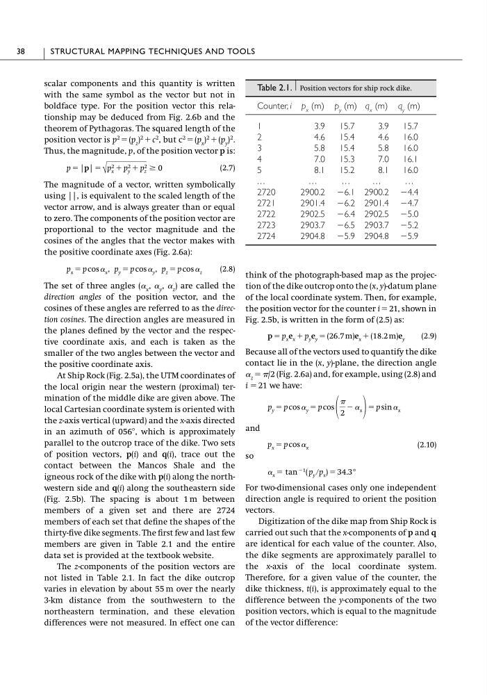
thirty-five dike segments. The first few and last few
members are given in Table 2.1 and the entire
data set is provided at the textbook website.
The z-components of the position vectors are
not listed in Table 2.1. In fact the dike outcrop
varies in elevation by about 55 m over the nearly
3-km distance from the southwestern to the
northeastern termination, and these elevation
differences were not measured. In effect one can
p x ϭ p cos ␣ x , p y ϭ p cos ␣ y , p z ϭ p cos ␣ z
p ϭ |p| ϭ √ p 2
x ϩ p 2
y ϩ p 2
z Ն 0
think of the photograph-based map as the projection of the dike outcrop onto the (x, y)-datum plane
of the local coordinate system. Then, for example,
the position vector for the counter i ϭ 21, shown in
Fig. 2.5b, is written in the form of (2.5) as:
(2.9)
Because all of the vectors used to quantify the dike
contact lie in the (x, y)-plane, the direction angle
␣ z ϭ /2 (Fig. 2.6a) and, for example, using (2.8) and
i ϭ 21 we have:
and
(2.10)
so
For two-dimensional cases only one independent
direction angle is required to orient the position
vectors.
Digitization of the dike map from Ship Rock is
carried out such that the x-components of p and q
are identical for each value of the counter. Also,
the dike segments are approximately parallel to
the x-axis of the local coordinate system.
Therefore, for a given value of the counter, the
dike thickness, t(i), is approximately equal to the
difference between the y-components of the two
position vectors, which is equal to the magnitude
of the vector difference:
␣ x ϭ tan Ϫ1 ( p y րp x ) ϭ 34.3°
p x ϭ p cos ␣ x
p y ϭ p cos ␣ y ϭ p cos
2
Ϫ ␣ x ϭ p sin ␣ x
p ϭ p x e x ϩ p y e y ϭ (26.7 m)e x ϩ (18.2 m)e y
38
STRUCTURAL MAPPING TECHNIQUES AND TOOLS
Table 2.1. Position vectors for ship rock dike.
Counter, i p x (m) p y (m) q x (m) q y (m)
1
3.9
15.7
3.9
15.7
2
4.6
15.4
4.6
16.0
3
5.8
15.4
5.8
16.0
4
7.0
15.3
7.0
16.1
5
8.1
15.2
8.1
16.0
. . .
. . .
. . .
. . .
. . .
2720
2900.2 Ϫ6.1 2900.2 Ϫ4.4
2721
2901.4 Ϫ6.2 2901.4 Ϫ4.7
2722
2902.5 Ϫ6.4 2902.5 Ϫ5.0
2723
2903.7 Ϫ6.5 2903.7 Ϫ5.2
2724
2904.8 Ϫ5.9 2904.8 Ϫ5.9
with the same symbol as the vector but not in
boldface type. For the position vector this relationship may be deduced from Fig. 2.6b and the
theorem of Pythagoras. The squared length of the
position vector is p
2 ϭ (p z )
2 ϩ c
2 , but c
2 ϭ (p x )
2 ϩ (p y )
2 .
Thus, the magnitude, p, of the position vector p is:
(2.7)
The magnitude of a vector, written symbolically
using ||, is equivalent to the scaled length of the
vector arrow, and is always greater than or equal
to zero. The components of the position vector are
proportional to the vector magnitude and the
cosines of the angles that the vector makes with
the positive coordinate axes (Fig. 2.6a):
(2.8)
The set of three angles (␣ x , ␣ y , ␣ z ) are called the
direction angles of the position vector, and the
cosines of these angles are referred to as the direction cosines. The direction angles are measured in
the planes defined by the vector and the respective coordinate axis, and each is taken as the
smaller of the two angles between the vector and
the positive coordinate axis.
At Ship Rock (Fig. 2.5a), the UTM coordinates of
the local origin near the western (proximal) termination of the middle dike are given above. The
local Cartesian coordinate system is oriented with
the z-axis vertical (upward) and the x-axis directed
in an azimuth of 056Њ, which is approximately
parallel to the outcrop trace of the dike. Two sets
of position vectors, p(i) and q(i), trace out the
contact between the Mancos Shale and the
igneous rock of the dike with p(i) along the northwestern side and q(i) along the southeastern side
(Fig. 2.5b). The spacing is about 1 m between
members of a given set and there are 2724
members of each set that define the shapes of the
thirty-five dike segments. The first few and last few
members are given in Table 2.1 and the entire
data set is provided at the textbook website.
The z-components of the position vectors are
not listed in Table 2.1. In fact the dike outcrop
varies in elevation by about 55 m over the nearly
3-km distance from the southwestern to the
northeastern termination, and these elevation
differences were not measured. In effect one can
p x ϭ p cos ␣ x , p y ϭ p cos ␣ y , p z ϭ p cos ␣ z
p ϭ |p| ϭ √ p 2
x ϩ p 2
y ϩ p 2
z Ն 0
think of the photograph-based map as the projection of the dike outcrop onto the (x, y)-datum plane
of the local coordinate system. Then, for example,
the position vector for the counter i ϭ 21, shown in
Fig. 2.5b, is written in the form of (2.5) as:
(2.9)
Because all of the vectors used to quantify the dike
contact lie in the (x, y)-plane, the direction angle
␣ z ϭ /2 (Fig. 2.6a) and, for example, using (2.8) and
i ϭ 21 we have:
and
(2.10)
so
For two-dimensional cases only one independent
direction angle is required to orient the position
vectors.
Digitization of the dike map from Ship Rock is
carried out such that the x-components of p and q
are identical for each value of the counter. Also,
the dike segments are approximately parallel to
the x-axis of the local coordinate system.
Therefore, for a given value of the counter, the
dike thickness, t(i), is approximately equal to the
difference between the y-components of the two
position vectors, which is equal to the magnitude
of the vector difference:
␣ x ϭ tan Ϫ1 ( p y րp x ) ϭ 34.3°
p x ϭ p cos ␣ x
p y ϭ p cos ␣ y ϭ p cos
2
Ϫ ␣ x ϭ p sin ␣ x
p ϭ p x e x ϩ p y e y ϭ (26.7 m)e x ϩ (18.2 m)e y
38
STRUCTURAL MAPPING TECHNIQUES AND TOOLS
Table 2.1. Position vectors for ship rock dike.
Counter, i p x (m) p y (m) q x (m) q y (m)
1
3.9
15.7
3.9
15.7
2
4.6
15.4
4.6
16.0
3
5.8
15.4
5.8
16.0
4
7.0
15.3
7.0
16.1
5
8.1
15.2
8.1
16.0
. . .
. . .
. . .
. . .
. . .
2720
2900.2 Ϫ6.1 2900.2 Ϫ4.4
2721
2901.4 Ϫ6.2 2901.4 Ϫ4.7
2722
2902.5 Ϫ6.4 2902.5 Ϫ5.0
2723
2903.7 Ϫ6.5 2903.7 Ϫ5.2
2724
2904.8 Ϫ5.9 2904.8 Ϫ5.9