

dike introduced some uncertainty in locating the
contact, this procedure generally provided the
required precision. A portion of the first photograph in the series is shown in Fig. 2.5b along with
the local coordinate system.
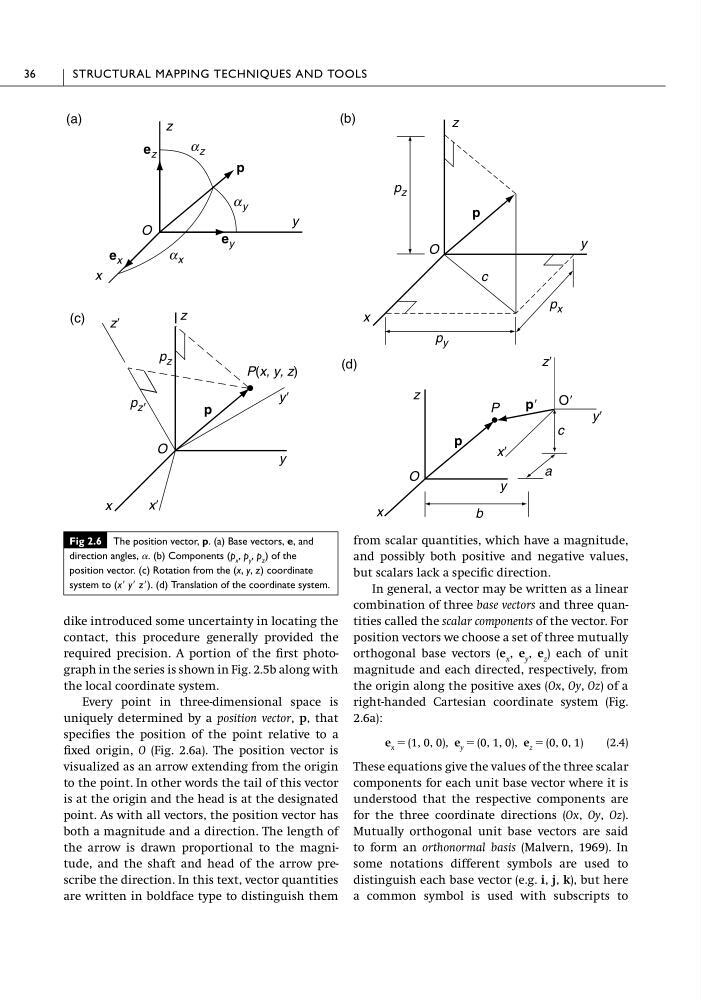
Every point in three-dimensional space is
uniquely determined by a position vector, p, that
specifies the position of the point relative to a
fixed origin, O (Fig. 2.6a). The position vector is
visualized as an arrow extending from the origin
to the point. In other words the tail of this vector
is at the origin and the head is at the designated
point. As with all vectors, the position vector has
both a magnitude and a direction. The length of
the arrow is drawn proportional to the magnitude, and the shaft and head of the arrow prescribe the direction. In this text, vector quantities
are written in boldface type to distinguish them
from scalar quantities, which have a magnitude,
and possibly both positive and negative values,
but scalars lack a specific direction.
In general, a vector may be written as a linear
combination of three base vectors and three quantities called the scalar components of the vector. For
position vectors we choose a set of three mutually
orthogonal base vectors (e x , e y , e z ) each of unit
magnitude and each directed, respectively, from
the origin along the positive axes (Ox, Oy, Oz) of a
right-handed Cartesian coordinate system (Fig.
2.6a):
(2.4)
These equations give the values of the three scalar
components for each unit base vector where it is
understood that the respective components are
for the three coordinate directions (Ox, Oy, Oz).
Mutually orthogonal unit base vectors are said
to form an orthonormal basis (Malvern, 1969). In
some notations different symbols are used to
distinguish each base vector (e.g. i, j, k), but here
a common symbol is used with subscripts to
e x ϭ (1, 0, 0), e y ϭ (0, 1, 0), e z ϭ (0, 0, 1)
36
STRUCTURAL MAPPING TECHNIQUES AND TOOLS
x
y
z
a z
(a)
O
(b)
p
x
y
z
p z
O
a y
a x
c
p
xЈ
zЈ
b
c
O
OЈ
yЈ
(d)
p
pЈ
x
y
z
(c)
O
p
yЈ
zЈ
xЈ
x
y
z
a
P(x, y, z)
P
p x
p y
p z
p zЈ
e y
e x
e z
Fig 2.6 The position vector, p. (a) Base vectors, e, and
direction angles, ␣. (b) Components (p x , p y , p z ) of the
position vector. (c) Rotation from the (x, y, z) coordinate
system to (xЈ yЈ zЈ). (d) Translation of the coordinate system.
contact, this procedure generally provided the
required precision. A portion of the first photograph in the series is shown in Fig. 2.5b along with
the local coordinate system.
Every point in three-dimensional space is
uniquely determined by a position vector, p, that
specifies the position of the point relative to a
fixed origin, O (Fig. 2.6a). The position vector is
visualized as an arrow extending from the origin
to the point. In other words the tail of this vector
is at the origin and the head is at the designated
point. As with all vectors, the position vector has
both a magnitude and a direction. The length of
the arrow is drawn proportional to the magnitude, and the shaft and head of the arrow prescribe the direction. In this text, vector quantities
are written in boldface type to distinguish them
from scalar quantities, which have a magnitude,
and possibly both positive and negative values,
but scalars lack a specific direction.
In general, a vector may be written as a linear
combination of three base vectors and three quantities called the scalar components of the vector. For
position vectors we choose a set of three mutually
orthogonal base vectors (e x , e y , e z ) each of unit
magnitude and each directed, respectively, from
the origin along the positive axes (Ox, Oy, Oz) of a
right-handed Cartesian coordinate system (Fig.
2.6a):
(2.4)
These equations give the values of the three scalar
components for each unit base vector where it is
understood that the respective components are
for the three coordinate directions (Ox, Oy, Oz).
Mutually orthogonal unit base vectors are said
to form an orthonormal basis (Malvern, 1969). In
some notations different symbols are used to
distinguish each base vector (e.g. i, j, k), but here
a common symbol is used with subscripts to
e x ϭ (1, 0, 0), e y ϭ (0, 1, 0), e z ϭ (0, 0, 1)
36
STRUCTURAL MAPPING TECHNIQUES AND TOOLS
x
y
z
a z
(a)
O
(b)
p
x
y
z
p z
O
a y
a x
c
p
xЈ
zЈ
b
c
O
OЈ
yЈ
(d)
p
pЈ
x
y
z
(c)
O
p
yЈ
zЈ
xЈ
x
y
z
a
P(x, y, z)
P
p x
p y
p z
p zЈ
e y
e x
e z
Fig 2.6 The position vector, p. (a) Base vectors, e, and
direction angles, ␣. (b) Components (p x , p y , p z ) of the
position vector. (c) Rotation from the (x, y, z) coordinate
system to (xЈ yЈ zЈ). (d) Translation of the coordinate system.