

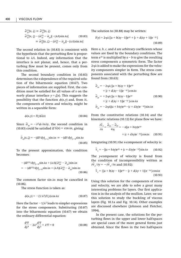
(10.83)
The second relation in (10.83) is consistent with
the hypothesis that the perturbing flow is proportional to A. Indeed, any information that the
interface is not planar, and, hence, that a perturbing flow must be present, comes only from
this condition.
The second boundary condition in (10.83)
determines the x-dependence of the required solution of the biharmonic equation (10.67). Two
pieces of information are supplied. First, the condition must be satisfied for all values of x on the
nearly planar interface y ϭ (x). This suggests the
possibility that the function (x, y) and, from it,
the components of stress and velocity, might be
written in a separable form:
(10.84)
Since
the second condition in
(10.83) could be satisfied if
giving:
(10.85)
To the present approximation, this condition
becomes:
(10.86)
The common factor sin x may be cancelled in
(10.86).
The stress function is taken as:
(10.87)
Here the factor Ϫ1/
2 leads to simpler expressions
for the stress components. Substituting (10.87)
into the biharmonic equation (10.67) we obtain
the ordinary differential equation:
(10.88)
d 4 F
dy 4 Ϫ 2 2 d 2 F
dy 2 ϩ 4 F ϭ 0
(x, y) ϭ Ϫ(1ր 2 ) F ( y) cos x
ϭ Ϫ (dF (2) րdy) yϭ0 sin x ϩ ( A)( (2)
xx Ϫ yy ) sin x
Ϫ (dF (1) րdy) yϭ0 sin x ϩ ( A)( (1)
xx Ϫ yy ) sin x
~ xy (x, ) ϭ Ϫ(dFրdy) yϭ sin x Х Ϫ(dFրdy) yϭ0 sin x
G(x) ϭ cos x,
~ xy ϭ ϪѨ 2 րѨxѨy,
(x, y) ϭ F( y)G(x)
Х
~ (2)
xy (x, ) Ϫ ( (2)
xx Ϫ yy )[Ϫ( A) sin x]
~ (1)
xy (x, ) Ϫ (
(1)
xx Ϫ yy )[Ϫ(A) sin x]
~ (1)
yy (x, ) Х
~ (2)
yy (x, )
The solution to (10.88) may be written:
(10.89)
Here a, b, c, and d are arbitrary coefficients whose
values are fixed by the boundary conditions. The
term e y is multiplied by a – b to give the resulting
stress components a symmetric form. The factor
2 is added to make the expressions for the velocity components simpler in form. The stress components associated with the perturbing flow are
found from (10.63):
(10.90)
From the constitutive relations (10.14) and the
kinematic relations (10.12) for plane flow we have:
(10.91)
Integrating (10.91) the x-component of velocity is:
(10.92)
The y-component of velocity is found from
the condition of incompressibility written as
and (10.92):
(10.93)
Using this solution for the components of stress
and velocity, we are able to solve a great many
interesting problems for layers. Our first application is in the analysis of the mullion. Later, we use
this solution to study the buckling of viscous
layers (Fig. 10.1a and Fig. 10.14). Other examples
are discussed elsewhere (Johnson and Fletcher,
1994).
In the present case, the solutions for the perturbing flows in the upper and lower half-spaces
are special cases of the more general forms just
obtained. Since the flows in the two half-spaces
e Ϫy }cosx
v
~ y ϭ {[a ϩ b(y Ϫ 1)]e y Ϫ [c ϩ d(y ϩ 1)]
Ѩv ~ y րѨy ϭ ϪѨv ~ x րѨx
v
~ x ϭ Ϫ[(a ϩ by)e y ϩ (c ϩ dy)e Ϫy ] sin x
ϩ (c ϩ dy)e Ϫy ] cosx
Ѩv ~ x
Ѩx
ϭ
~ xx Ϫ
~ yy
4
ϭ Ϫ[(a ϩ by)e y
~ xy ϭ Ϫ2[(a ϩ by)e y Ϫ(c ϩ dy)e Ϫy ] sin x
ϩ [c ϩ d(y ϩ 1)]e Ϫy }cos x
~ yy ϭ ϩ2{[a ϩ b(yϪ1)]e y
ϩ [c ϩ d(yϪ1)]e Ϫy }cosx
~ xx ϭ Ϫ2{[a ϩ b(y ϩ 1)]e y
F( y) ϭ 2{[a ϩ b(yϪ1)]e y ϩ [c ϩ d(y ϩ 1)]e Ϫy }
400
VISCOUS FLOW
The second relation in (10.83) is consistent with
the hypothesis that the perturbing flow is proportional to A. Indeed, any information that the
interface is not planar, and, hence, that a perturbing flow must be present, comes only from
this condition.
The second boundary condition in (10.83)
determines the x-dependence of the required solution of the biharmonic equation (10.67). Two
pieces of information are supplied. First, the condition must be satisfied for all values of x on the
nearly planar interface y ϭ (x). This suggests the
possibility that the function (x, y) and, from it,
the components of stress and velocity, might be
written in a separable form:
(10.84)
Since
the second condition in
(10.83) could be satisfied if
giving:
(10.85)
To the present approximation, this condition
becomes:
(10.86)
The common factor sin x may be cancelled in
(10.86).
The stress function is taken as:
(10.87)
Here the factor Ϫ1/
2 leads to simpler expressions
for the stress components. Substituting (10.87)
into the biharmonic equation (10.67) we obtain
the ordinary differential equation:
(10.88)
d 4 F
dy 4 Ϫ 2 2 d 2 F
dy 2 ϩ 4 F ϭ 0
(x, y) ϭ Ϫ(1ր 2 ) F ( y) cos x
ϭ Ϫ (dF (2) րdy) yϭ0 sin x ϩ ( A)( (2)
xx Ϫ yy ) sin x
Ϫ (dF (1) րdy) yϭ0 sin x ϩ ( A)( (1)
xx Ϫ yy ) sin x
~ xy (x, ) ϭ Ϫ(dFրdy) yϭ sin x Х Ϫ(dFրdy) yϭ0 sin x
G(x) ϭ cos x,
~ xy ϭ ϪѨ 2 րѨxѨy,
(x, y) ϭ F( y)G(x)
Х
~ (2)
xy (x, ) Ϫ ( (2)
xx Ϫ yy )[Ϫ( A) sin x]
~ (1)
xy (x, ) Ϫ (
(1)
xx Ϫ yy )[Ϫ(A) sin x]
~ (1)
yy (x, ) Х
~ (2)
yy (x, )
The solution to (10.88) may be written:
(10.89)
Here a, b, c, and d are arbitrary coefficients whose
values are fixed by the boundary conditions. The
term e y is multiplied by a – b to give the resulting
stress components a symmetric form. The factor
2 is added to make the expressions for the velocity components simpler in form. The stress components associated with the perturbing flow are
found from (10.63):
(10.90)
From the constitutive relations (10.14) and the
kinematic relations (10.12) for plane flow we have:
(10.91)
Integrating (10.91) the x-component of velocity is:
(10.92)
The y-component of velocity is found from
the condition of incompressibility written as
and (10.92):
(10.93)
Using this solution for the components of stress
and velocity, we are able to solve a great many
interesting problems for layers. Our first application is in the analysis of the mullion. Later, we use
this solution to study the buckling of viscous
layers (Fig. 10.1a and Fig. 10.14). Other examples
are discussed elsewhere (Johnson and Fletcher,
1994).
In the present case, the solutions for the perturbing flows in the upper and lower half-spaces
are special cases of the more general forms just
obtained. Since the flows in the two half-spaces
e Ϫy }cosx
v
~ y ϭ {[a ϩ b(y Ϫ 1)]e y Ϫ [c ϩ d(y ϩ 1)]
Ѩv ~ y րѨy ϭ ϪѨv ~ x րѨx
v
~ x ϭ Ϫ[(a ϩ by)e y ϩ (c ϩ dy)e Ϫy ] sin x
ϩ (c ϩ dy)e Ϫy ] cosx
Ѩv ~ x
Ѩx
ϭ
~ xx Ϫ
~ yy
4
ϭ Ϫ[(a ϩ by)e y
~ xy ϭ Ϫ2[(a ϩ by)e y Ϫ(c ϩ dy)e Ϫy ] sin x
ϩ [c ϩ d(y ϩ 1)]e Ϫy }cos x
~ yy ϭ ϩ2{[a ϩ b(yϪ1)]e y
ϩ [c ϩ d(yϪ1)]e Ϫy }cosx
~ xx ϭ Ϫ2{[a ϩ b(y ϩ 1)]e y
F( y) ϭ 2{[a ϩ b(yϪ1)]e y ϩ [c ϩ d(y ϩ 1)]e Ϫy }
400
VISCOUS FLOW