

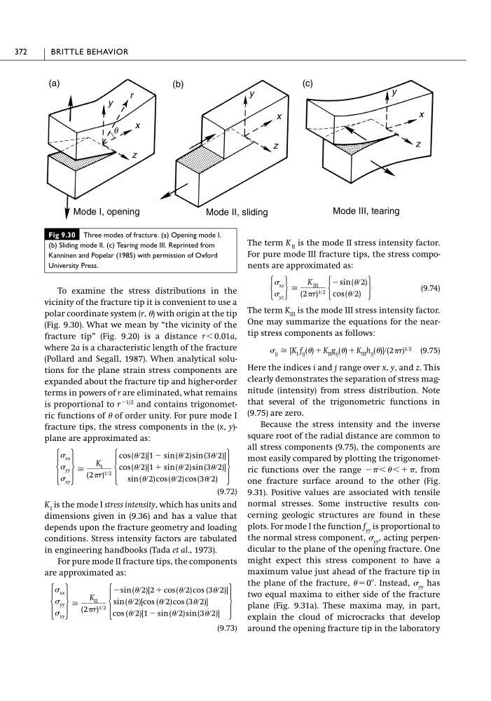
To examine the stress distributions in the
vicinity of the fracture tip it is convenient to use a
polar coordinate system (r, ) with origin at the tip
(Fig. 9.30). What we mean by “the vicinity of the
fracture tip” (Fig. 9.20) is a distance r Ͻ 0.01a,
where 2a is a characteristic length of the fracture
(Pollard and Segall, 1987). When analytical solutions for the plane strain stress components are
expanded about the fracture tip and higher-order
terms in powers of r are eliminated, what remains
is proportional to r
Ϫ1/2 and contains trigonometric functions of of order unity. For pure mode I
fracture tips, the stress components in the (x, y)plane are approximated as:
(9.72)
K I is the mode I stress intensity, which has units and
dimensions given in (9.36) and has a value that
depends upon the fracture geometry and loading
conditions. Stress intensity factors are tabulated
in engineering handbooks (Tada et al., 1973).
For pure mode II fracture tips, the components
are approximated as:
(9.73)
Ά
xx
yy
xy
·
Х
K II
(2r) 1ր2 Ά
Ϫsin (ր2)[2 ϩ cos (ր2) cos (3ր2)]
sin (ր2)[cos (ր2) cos (3ր2)]
cos (ր2)[1 Ϫ sin (ր2) sin (3ր2)]
·
Ά
xx
yy
xy
·
Х
K I
(2r) 1ր2 Ά
cos (ր2)[1 Ϫ sin (ր2) sin (3ր2)]
cos (ր2)[1 ϩ sin (ր2) sin (3ր2)]
sin (ր2) cos (ր2) cos (3ր2)
·
The term K II is the mode II stress intensity factor.
For pure mode III fracture tips, the stress components are approximated as:
(9.74)
The term K III is the mode III stress intensity factor.
One may summarize the equations for the neartip stress components as follows:
(9.75)
Here the indices i and j range over x, y, and z. This
clearly demonstrates the separation of stress magnitude (intensity) from stress distribution. Note
that several of the trigonometric functions in
(9.75) are zero.
Because the stress intensity and the inverse
square root of the radial distance are common to
all stress components (9.75), the components are
most easily compared by plotting the trigonometric functions over the range Ϫ Ͻ Ͻϩ, from
one fracture surface around to the other (Fig.
9.31). Positive values are associated with tensile
normal stresses. Some instructive results concerning geologic structures are found in these
plots. For mode I the function f yy is proportional to
the normal stress component, yy , acting perpendicular to the plane of the opening fracture. One
might expect this stress component to have a
maximum value just ahead of the fracture tip in
the plane of the fracture, ϭ 0Њ. Instead, yy has
two equal maxima to either side of the fracture
plane (Fig. 9.31a). These maxima may, in part,
explain the cloud of microcracks that develop
around the opening fracture tip in the laboratory
ij Х [K I f ij () ϩ K II g ij () ϩ K III h ij ()]ր(2r) 1ր2
Ά
xz
yz ·
Х
K III
(2r) 1ր2 Ά
Ϫ sin (ր2)
cos (ր2) ·
372
BRITTLE BEHAVIOR
Fig 9.30 Three modes of fracture. (a) Opening mode I.
(b) Sliding mode II. (c) Tearing mode III. Reprinted from
Kanninen and Popelar (1985) with permission of Oxford
University Press.
(a)
(b)
(c)
x
y
z
x
y
z
x
y
z
r
u
Mode I, opening
Mode II, sliding
Mode III, tearing
vicinity of the fracture tip it is convenient to use a
polar coordinate system (r, ) with origin at the tip
(Fig. 9.30). What we mean by “the vicinity of the
fracture tip” (Fig. 9.20) is a distance r Ͻ 0.01a,
where 2a is a characteristic length of the fracture
(Pollard and Segall, 1987). When analytical solutions for the plane strain stress components are
expanded about the fracture tip and higher-order
terms in powers of r are eliminated, what remains
is proportional to r
Ϫ1/2 and contains trigonometric functions of of order unity. For pure mode I
fracture tips, the stress components in the (x, y)plane are approximated as:
(9.72)
K I is the mode I stress intensity, which has units and
dimensions given in (9.36) and has a value that
depends upon the fracture geometry and loading
conditions. Stress intensity factors are tabulated
in engineering handbooks (Tada et al., 1973).
For pure mode II fracture tips, the components
are approximated as:
(9.73)
Ά
xx
yy
xy
·
Х
K II
(2r) 1ր2 Ά
Ϫsin (ր2)[2 ϩ cos (ր2) cos (3ր2)]
sin (ր2)[cos (ր2) cos (3ր2)]
cos (ր2)[1 Ϫ sin (ր2) sin (3ր2)]
·
Ά
xx
yy
xy
·
Х
K I
(2r) 1ր2 Ά
cos (ր2)[1 Ϫ sin (ր2) sin (3ր2)]
cos (ր2)[1 ϩ sin (ր2) sin (3ր2)]
sin (ր2) cos (ր2) cos (3ր2)
·
The term K II is the mode II stress intensity factor.
For pure mode III fracture tips, the stress components are approximated as:
(9.74)
The term K III is the mode III stress intensity factor.
One may summarize the equations for the neartip stress components as follows:
(9.75)
Here the indices i and j range over x, y, and z. This
clearly demonstrates the separation of stress magnitude (intensity) from stress distribution. Note
that several of the trigonometric functions in
(9.75) are zero.
Because the stress intensity and the inverse
square root of the radial distance are common to
all stress components (9.75), the components are
most easily compared by plotting the trigonometric functions over the range Ϫ Ͻ Ͻϩ, from
one fracture surface around to the other (Fig.
9.31). Positive values are associated with tensile
normal stresses. Some instructive results concerning geologic structures are found in these
plots. For mode I the function f yy is proportional to
the normal stress component, yy , acting perpendicular to the plane of the opening fracture. One
might expect this stress component to have a
maximum value just ahead of the fracture tip in
the plane of the fracture, ϭ 0Њ. Instead, yy has
two equal maxima to either side of the fracture
plane (Fig. 9.31a). These maxima may, in part,
explain the cloud of microcracks that develop
around the opening fracture tip in the laboratory
ij Х [K I f ij () ϩ K II g ij () ϩ K III h ij ()]ր(2r) 1ր2
Ά
xz
yz ·
Х
K III
(2r) 1ր2 Ά
Ϫ sin (ր2)
cos (ր2) ·
372
BRITTLE BEHAVIOR
Fig 9.30 Three modes of fracture. (a) Opening mode I.
(b) Sliding mode II. (c) Tearing mode III. Reprinted from
Kanninen and Popelar (1985) with permission of Oxford
University Press.
(a)
(b)
(c)
x
y
z
x
y
z
x
y
z
r
u
Mode I, opening
Mode II, sliding
Mode III, tearing