

stress, but they disregarded the shape of the hole
and focused their attention on the cross-sectional
area of material outside the hole (Gordon, 1976).
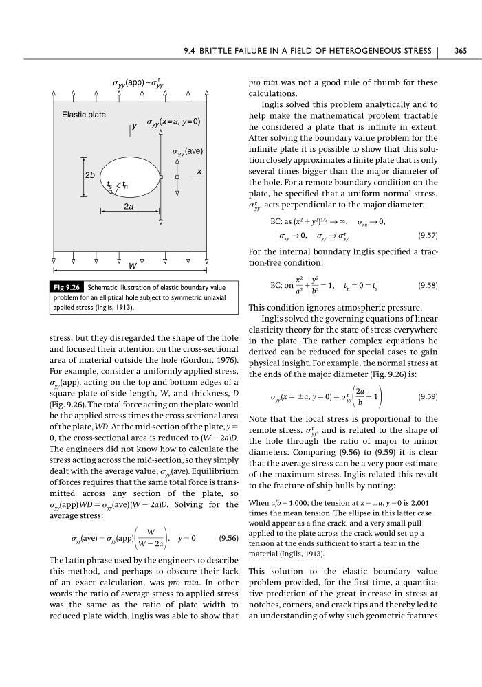
For example, consider a uniformly applied stress,
yy (app), acting on the top and bottom edges of a
square plate of side length, W, and thickness, D
(Fig. 9.26). The total force acting on the plate would
be the applied stress times the cross-sectional area
of the plate, WD. At the mid-section of the plate, y ϭ
0, the cross-sectional area is reduced to (W Ϫ 2a)D.
The engineers did not know how to calculate the
stress acting across the mid-section, so they simply
dealt with the average value, yy (ave). Equilibrium
of forces requires that the same total force is transmitted across any section of the plate, so
Solving for the
average stress:
(9.56)
The Latin phrase used by the engineers to describe
this method, and perhaps to obscure their lack
of an exact calculation, was pro rata. In other
words the ratio of average stress to applied stress
was the same as the ratio of plate width to
reduced plate width. Inglis was able to show that
yy (ave) ϭ yy (app)
W
W Ϫ 2a
, y ϭ 0
yy (app) WD ϭ yy (ave) (W Ϫ 2a)D.
pro rata was not a good rule of thumb for these
calculations.
Inglis solved this problem analytically and to
help make the mathematical problem tractable
he considered a plate that is infinite in extent.
After solving the boundary value problem for the
infinite plate it is possible to show that this solution closely approximates a finite plate that is only
several times bigger than the major diameter of
the hole. For a remote boundary condition on the
plate, he specified that a uniform normal stress,
acts perpendicular to the major diameter:
(9.57)
For the internal boundary Inglis specified a traction-free condition:
(9.58)
This condition ignores atmospheric pressure.
Inglis solved the governing equations of linear
elasticity theory for the state of stress everywhere
in the plate. The rather complex equations he
derived can be reduced for special cases to gain
physical insight. For example, the normal stress at
the ends of the major diameter (Fig. 9.26) is:
(9.59)
Note that the local stress is proportional to the
remote stress,
and is related to the shape of
the hole through the ratio of major to minor
diameters. Comparing (9.56) to (9.59) it is clear
that the average stress can be a very poor estimate
of the maximum stress. Inglis related this result
to the fracture of ship hulls by noting:
When a/b ϭ 1,000, the tension at xϭϮa, yϭ0 is 2,001
times the mean tension. The ellipse in this latter case
would appear as a fine crack, and a very small pull
applied to the plate across the crack would set up a
tension at the ends sufficient to start a tear in the
material (Inglis, 1913).
This solution to the elastic boundary value
problem provided, for the first time, a quantitative prediction of the great increase in stress at
notches, corners, and crack tips and thereby led to
an understanding of why such geometric features
r
yy ,
yy (x ϭ Ϯa, y ϭ 0) ϭ r
yy
2a
b
ϩ 1
BC: on
x 2
a 2 ϩ
y 2
b 2 ϭ 1, t n ϭ 0 ϭ t s
xy → 0, yy → r
yy
BC: as (x 2 ϩ y 2 ) 1ր2 → ϱ, xx → 0,
r
yy ,
9.4 BRITTLE FAILURE IN A FIELD OF HETEROGENEOUS STRESS
365
Fig 9.26 Schematic illustration of elastic boundary value
problem for an elliptical hole subject to symmetric uniaxial
applied stress (Inglis, 1913).
y
x
2b
2a
W
t s t n
Elastic plate
s yy (x = a, y = 0)
s yy (ave)
s yy (app) ~ s yy
r
and focused their attention on the cross-sectional
area of material outside the hole (Gordon, 1976).
For example, consider a uniformly applied stress,
yy (app), acting on the top and bottom edges of a
square plate of side length, W, and thickness, D
(Fig. 9.26). The total force acting on the plate would
be the applied stress times the cross-sectional area
of the plate, WD. At the mid-section of the plate, y ϭ
0, the cross-sectional area is reduced to (W Ϫ 2a)D.
The engineers did not know how to calculate the
stress acting across the mid-section, so they simply
dealt with the average value, yy (ave). Equilibrium
of forces requires that the same total force is transmitted across any section of the plate, so
Solving for the
average stress:
(9.56)
The Latin phrase used by the engineers to describe
this method, and perhaps to obscure their lack
of an exact calculation, was pro rata. In other
words the ratio of average stress to applied stress
was the same as the ratio of plate width to
reduced plate width. Inglis was able to show that
yy (ave) ϭ yy (app)
W
W Ϫ 2a
, y ϭ 0
yy (app) WD ϭ yy (ave) (W Ϫ 2a)D.
pro rata was not a good rule of thumb for these
calculations.
Inglis solved this problem analytically and to
help make the mathematical problem tractable
he considered a plate that is infinite in extent.
After solving the boundary value problem for the
infinite plate it is possible to show that this solution closely approximates a finite plate that is only
several times bigger than the major diameter of
the hole. For a remote boundary condition on the
plate, he specified that a uniform normal stress,
acts perpendicular to the major diameter:
(9.57)
For the internal boundary Inglis specified a traction-free condition:
(9.58)
This condition ignores atmospheric pressure.
Inglis solved the governing equations of linear
elasticity theory for the state of stress everywhere
in the plate. The rather complex equations he
derived can be reduced for special cases to gain
physical insight. For example, the normal stress at
the ends of the major diameter (Fig. 9.26) is:
(9.59)
Note that the local stress is proportional to the
remote stress,
and is related to the shape of
the hole through the ratio of major to minor
diameters. Comparing (9.56) to (9.59) it is clear
that the average stress can be a very poor estimate
of the maximum stress. Inglis related this result
to the fracture of ship hulls by noting:
When a/b ϭ 1,000, the tension at xϭϮa, yϭ0 is 2,001
times the mean tension. The ellipse in this latter case
would appear as a fine crack, and a very small pull
applied to the plate across the crack would set up a
tension at the ends sufficient to start a tear in the
material (Inglis, 1913).
This solution to the elastic boundary value
problem provided, for the first time, a quantitative prediction of the great increase in stress at
notches, corners, and crack tips and thereby led to
an understanding of why such geometric features
r
yy ,
yy (x ϭ Ϯa, y ϭ 0) ϭ r
yy
2a
b
ϩ 1
BC: on
x 2
a 2 ϩ
y 2
b 2 ϭ 1, t n ϭ 0 ϭ t s
xy → 0, yy → r
yy
BC: as (x 2 ϩ y 2 ) 1ր2 → ϱ, xx → 0,
r
yy ,
9.4 BRITTLE FAILURE IN A FIELD OF HETEROGENEOUS STRESS
365
Fig 9.26 Schematic illustration of elastic boundary value
problem for an elliptical hole subject to symmetric uniaxial
applied stress (Inglis, 1913).
y
x
2b
2a
W
t s t n
Elastic plate
s yy (x = a, y = 0)
s yy (ave)
s yy (app) ~ s yy
r