

testing machine that can load rock samples to
their limiting values of stress. Furthermore, the
load-bearing members of the machine can be
designed with greater cross-sectional area than
the sample, so the net force induces a lesser stress
in the machine than in the sample. An example
of such a machine is shown in Fig. 8.25. The outer
steel frame supports the load transmitted
through the sample from a mobile platen to a
fixed platen. A hydraulic pump provides pressure
to move a piston that is attached to the mobile
platen. A computer controls the flow of the
hydraulic fluid (and thereby the motion of this
platen) based upon electronic readings from a
displacement transducer and load cell that
monitor the deformation and loading of the
sample.
Data from such tests on cylindrical samples of
rock usually are recorded on graphs of axial stress,
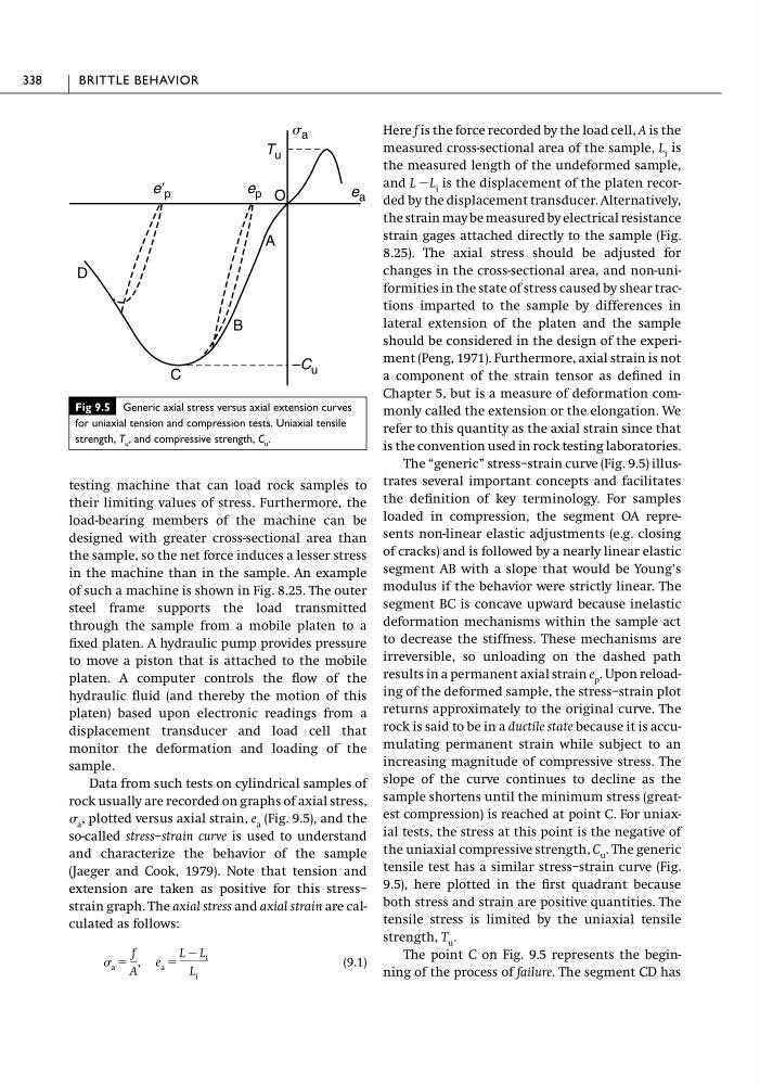
a , plotted versus axial strain, e a (Fig. 9.5), and the
so-called stress–strain curve is used to understand
and characterize the behavior of the sample
(Jaeger and Cook, 1979). Note that tension and
extension are taken as positive for this stress–
strain graph. The axial stress and axial strain are calculated as follows:
(9.1)
a ϭ
f
A
,e a ϭ
L Ϫ L i
L i
Here f is the force recorded by the load cell, A is the
measured cross-sectional area of the sample, L i is
the measured length of the undeformed sample,
and LϪL i is the displacement of the platen recorded by the displacement transducer. Alternatively,
the strain may be measured by electrical resistance
strain gages attached directly to the sample (Fig.
8.25). The axial stress should be adjusted for
changes in the cross-sectional area, and non-uniformities in the state of stress caused by shear tractions imparted to the sample by differences in
lateral extension of the platen and the sample
should be considered in the design of the experiment (Peng, 1971). Furthermore, axial strain is not
a component of the strain tensor as defined in
Chapter 5, but is a measure of deformation commonly called the extension or the elongation. We
refer to this quantity as the axial strain since that
is the convention used in rock testing laboratories.
The “generic” stress–strain curve (Fig. 9.5) illustrates several important concepts and facilitates
the definition of key terminology. For samples
loaded in compression, the segment OA represents non-linear elastic adjustments (e.g. closing
of cracks) and is followed by a nearly linear elastic
segment AB with a slope that would be Young’s
modulus if the behavior were strictly linear. The
segment BC is concave upward because inelastic
deformation mechanisms within the sample act
to decrease the stiffness. These mechanisms are
irreversible, so unloading on the dashed path
results in a permanent axial strain e p . Upon reloading of the deformed sample, the stress–strain plot
returns approximately to the original curve. The
rock is said to be in a ductile state because it is accumulating permanent strain while subject to an
increasing magnitude of compressive stress. The
slope of the curve continues to decline as the
sample shortens until the minimum stress (greatest compression) is reached at point C. For uniaxial tests, the stress at this point is the negative of
the uniaxial compressive strength, C u . The generic
tensile test has a similar stress–strain curve (Fig.
9.5), here plotted in the first quadrant because
both stress and strain are positive quantities. The
tensile stress is limited by the uniaxial tensile
strength, T u .
The point C on Fig. 9.5 represents the beginning of the process of failure. The segment CD has
338
BRITTLE BEHAVIOR
Fig 9.5 Generic axial stress versus axial extension curves
for uniaxial tension and compression tests. Uniaxial tensile
strength, T u , and compressive strength, C u .
T u
–C u
s a
e a
O
A
B
C
D
eЈ p
e p
their limiting values of stress. Furthermore, the
load-bearing members of the machine can be
designed with greater cross-sectional area than
the sample, so the net force induces a lesser stress
in the machine than in the sample. An example
of such a machine is shown in Fig. 8.25. The outer
steel frame supports the load transmitted
through the sample from a mobile platen to a
fixed platen. A hydraulic pump provides pressure
to move a piston that is attached to the mobile
platen. A computer controls the flow of the
hydraulic fluid (and thereby the motion of this
platen) based upon electronic readings from a
displacement transducer and load cell that
monitor the deformation and loading of the
sample.
Data from such tests on cylindrical samples of
rock usually are recorded on graphs of axial stress,
a , plotted versus axial strain, e a (Fig. 9.5), and the
so-called stress–strain curve is used to understand
and characterize the behavior of the sample
(Jaeger and Cook, 1979). Note that tension and
extension are taken as positive for this stress–
strain graph. The axial stress and axial strain are calculated as follows:
(9.1)
a ϭ
f
A
,e a ϭ
L Ϫ L i
L i
Here f is the force recorded by the load cell, A is the
measured cross-sectional area of the sample, L i is
the measured length of the undeformed sample,
and LϪL i is the displacement of the platen recorded by the displacement transducer. Alternatively,
the strain may be measured by electrical resistance
strain gages attached directly to the sample (Fig.
8.25). The axial stress should be adjusted for
changes in the cross-sectional area, and non-uniformities in the state of stress caused by shear tractions imparted to the sample by differences in
lateral extension of the platen and the sample
should be considered in the design of the experiment (Peng, 1971). Furthermore, axial strain is not
a component of the strain tensor as defined in
Chapter 5, but is a measure of deformation commonly called the extension or the elongation. We
refer to this quantity as the axial strain since that
is the convention used in rock testing laboratories.
The “generic” stress–strain curve (Fig. 9.5) illustrates several important concepts and facilitates
the definition of key terminology. For samples
loaded in compression, the segment OA represents non-linear elastic adjustments (e.g. closing
of cracks) and is followed by a nearly linear elastic
segment AB with a slope that would be Young’s
modulus if the behavior were strictly linear. The
segment BC is concave upward because inelastic
deformation mechanisms within the sample act
to decrease the stiffness. These mechanisms are
irreversible, so unloading on the dashed path
results in a permanent axial strain e p . Upon reloading of the deformed sample, the stress–strain plot
returns approximately to the original curve. The
rock is said to be in a ductile state because it is accumulating permanent strain while subject to an
increasing magnitude of compressive stress. The
slope of the curve continues to decline as the
sample shortens until the minimum stress (greatest compression) is reached at point C. For uniaxial tests, the stress at this point is the negative of
the uniaxial compressive strength, C u . The generic
tensile test has a similar stress–strain curve (Fig.
9.5), here plotted in the first quadrant because
both stress and strain are positive quantities. The
tensile stress is limited by the uniaxial tensile
strength, T u .
The point C on Fig. 9.5 represents the beginning of the process of failure. The segment CD has
338
BRITTLE BEHAVIOR
Fig 9.5 Generic axial stress versus axial extension curves
for uniaxial tension and compression tests. Uniaxial tensile
strength, T u , and compressive strength, C u .
T u
–C u
s a
e a
O
A
B
C
D
eЈ p
e p