

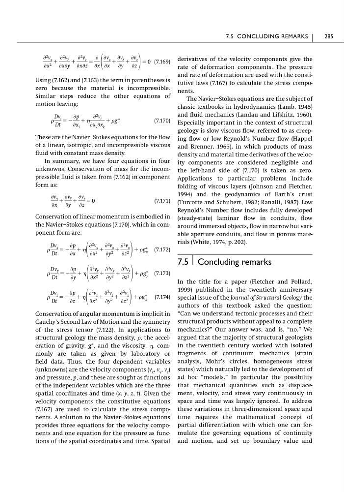
(7.169)
Using (7.162) and (7.163) the term in parentheses is
zero because the material is incompressible.
Similar steps reduce the other equations of
motion leaving:
(7.170)
These are the Navier–Stokes equations for the flow
of a linear, isotropic, and incompressible viscous
fluid with constant mass density.
In summary, we have four equations in four
unknowns. Conservation of mass for the incompressible fluid is taken from (7.162) in component
form as:
(7.171)
Conservation of linear momentum is embodied in
the Navier–Stokes equations (7.170), which in component form are:
(7.172)
(7.173)
(7.174)
Conservation of angular momentum is implicit in
Cauchy’s Second Law of Motion and the symmetry
of the stress tensor (7.122). In applications to
structural geology the mass density, , the acceleration of gravity, g*, and the viscosity, , commonly are taken as given by laboratory or
field data. Thus, the four dependent variables
(unknowns) are the velocity components (v x , v y , v z )
and pressure, p, and these are sought as functions
of the independent variables which are the three
spatial coordinates and time (x, y, z, t). Given the
velocity components the constitutive equations
(7.167) are used to calculate the stress components. A solution to the Navier–Stokes equations
provides three equations for the velocity components and one equation for the pressure as functions of the spatial coordinates and time. Spatial
Dv z
Dt
ϭ Ϫ
Ѩp
Ѩz
ϩ
Ѩ 2 v z
Ѩx 2 ϩ
Ѩ 2 v z
Ѩy 2 ϩ
Ѩ 2 v z
Ѩz 2
ϩ g* z
Dv y
Dt
ϭ Ϫ
Ѩp
Ѩy
ϩ
Ѩ 2 v y
Ѩx 2 ϩ
Ѩ 2 v y
Ѩy 2 ϩ
Ѩ 2 v y
Ѩz 2 ϩ g* y
Dv x
Dt
ϭ Ϫ
Ѩp
Ѩx
ϩ
Ѩ 2 v x
Ѩx 2 ϩ
Ѩ 2 v x
Ѩy 2 ϩ
Ѩ 2 v x
Ѩz 2
ϩ g* x
Ѩv x
Ѩx
ϩ
Ѩv y
Ѩy
ϩ
Ѩv z
Ѩz
ϭ 0
Dv i
Dt
ϭ Ϫ
Ѩp
Ѩx i
ϩ
Ѩ 2 v i
Ѩx k Ѩx k
ϩ g * i
Ѩ 2 v x
Ѩx 2 ϩ
Ѩ 2 v y
ѨxѨy
ϩ
Ѩ 2 v z
ѨxѨz
ϭ
Ѩ
Ѩx
Ѩv x
Ѩx
ϩ
Ѩv y
Ѩy
ϩ
Ѩv z
Ѩz
ϭ 0
derivatives of the velocity components give the
rate of deformation components. The pressure
and rate of deformation are used with the constitutive laws (7.167) to calculate the stress components.
The Navier–Stokes equations are the subject of
classic textbooks in hydrodynamics (Lamb, 1945)
and fluid mechanics (Landau and Lifshitz, 1960).
Especially important in the context of structural
geology is slow viscous flow, referred to as creeping flow or low Reynold’s Number flow (Happel
and Brenner, 1965), in which products of mass
density and material time derivatives of the velocity components are considered negligible and
the left-hand side of (7.170) is taken as zero.
Applications to particular problems include
folding of viscous layers (Johnson and Fletcher,
1994) and the geodynamics of Earth’s crust
(Turcotte and Schubert, 1982; Ranalli, 1987). Low
Reynold’s Number flow includes fully developed
(steady-state) laminar flow in conduits, flow
around immersed objects, flow in narrow but variable aperture conduits, and flow in porous materials (White, 1974, p. 202).
7.5 Concluding remarks
In the title for a paper (Fletcher and Pollard,
1999) published in the twentieth anniversary
special issue of the Journal of Structural Geology the
authors of this textbook asked the question:
“Can we understand tectonic processes and their
structural products without appeal to a complete
mechanics?” Our answer was, and is, “no.” We
argued that the majority of structural geologists
in the twentieth century worked with isolated
fragments of continuum mechanics (strain
analysis, Mohr’s circles, homogeneous stress
states) which naturally led to the development of
ad hoc “models.” In particular the possibility
that mechanical quantities such as displacement, velocity, and stress vary continuously in
space and time was largely ignored. To address
these variations in three-dimensional space and
time requires the mathematical concept of
partial differentiation with which one can formulate the governing equations of continuity
and motion, and set up boundary value and
7.5 CONCLUDING REMARKS
285
Using (7.162) and (7.163) the term in parentheses is
zero because the material is incompressible.
Similar steps reduce the other equations of
motion leaving:
(7.170)
These are the Navier–Stokes equations for the flow
of a linear, isotropic, and incompressible viscous
fluid with constant mass density.
In summary, we have four equations in four
unknowns. Conservation of mass for the incompressible fluid is taken from (7.162) in component
form as:
(7.171)
Conservation of linear momentum is embodied in
the Navier–Stokes equations (7.170), which in component form are:
(7.172)
(7.173)
(7.174)
Conservation of angular momentum is implicit in
Cauchy’s Second Law of Motion and the symmetry
of the stress tensor (7.122). In applications to
structural geology the mass density, , the acceleration of gravity, g*, and the viscosity, , commonly are taken as given by laboratory or
field data. Thus, the four dependent variables
(unknowns) are the velocity components (v x , v y , v z )
and pressure, p, and these are sought as functions
of the independent variables which are the three
spatial coordinates and time (x, y, z, t). Given the
velocity components the constitutive equations
(7.167) are used to calculate the stress components. A solution to the Navier–Stokes equations
provides three equations for the velocity components and one equation for the pressure as functions of the spatial coordinates and time. Spatial
Dv z
Dt
ϭ Ϫ
Ѩp
Ѩz
ϩ
Ѩ 2 v z
Ѩx 2 ϩ
Ѩ 2 v z
Ѩy 2 ϩ
Ѩ 2 v z
Ѩz 2
ϩ g* z
Dv y
Dt
ϭ Ϫ
Ѩp
Ѩy
ϩ
Ѩ 2 v y
Ѩx 2 ϩ
Ѩ 2 v y
Ѩy 2 ϩ
Ѩ 2 v y
Ѩz 2 ϩ g* y
Dv x
Dt
ϭ Ϫ
Ѩp
Ѩx
ϩ
Ѩ 2 v x
Ѩx 2 ϩ
Ѩ 2 v x
Ѩy 2 ϩ
Ѩ 2 v x
Ѩz 2
ϩ g* x
Ѩv x
Ѩx
ϩ
Ѩv y
Ѩy
ϩ
Ѩv z
Ѩz
ϭ 0
Dv i
Dt
ϭ Ϫ
Ѩp
Ѩx i
ϩ
Ѩ 2 v i
Ѩx k Ѩx k
ϩ g * i
Ѩ 2 v x
Ѩx 2 ϩ
Ѩ 2 v y
ѨxѨy
ϩ
Ѩ 2 v z
ѨxѨz
ϭ
Ѩ
Ѩx
Ѩv x
Ѩx
ϩ
Ѩv y
Ѩy
ϩ
Ѩv z
Ѩz
ϭ 0
derivatives of the velocity components give the
rate of deformation components. The pressure
and rate of deformation are used with the constitutive laws (7.167) to calculate the stress components.
The Navier–Stokes equations are the subject of
classic textbooks in hydrodynamics (Lamb, 1945)
and fluid mechanics (Landau and Lifshitz, 1960).
Especially important in the context of structural
geology is slow viscous flow, referred to as creeping flow or low Reynold’s Number flow (Happel
and Brenner, 1965), in which products of mass
density and material time derivatives of the velocity components are considered negligible and
the left-hand side of (7.170) is taken as zero.
Applications to particular problems include
folding of viscous layers (Johnson and Fletcher,
1994) and the geodynamics of Earth’s crust
(Turcotte and Schubert, 1982; Ranalli, 1987). Low
Reynold’s Number flow includes fully developed
(steady-state) laminar flow in conduits, flow
around immersed objects, flow in narrow but variable aperture conduits, and flow in porous materials (White, 1974, p. 202).
7.5 Concluding remarks
In the title for a paper (Fletcher and Pollard,
1999) published in the twentieth anniversary
special issue of the Journal of Structural Geology the
authors of this textbook asked the question:
“Can we understand tectonic processes and their
structural products without appeal to a complete
mechanics?” Our answer was, and is, “no.” We
argued that the majority of structural geologists
in the twentieth century worked with isolated
fragments of continuum mechanics (strain
analysis, Mohr’s circles, homogeneous stress
states) which naturally led to the development of
ad hoc “models.” In particular the possibility
that mechanical quantities such as displacement, velocity, and stress vary continuously in
space and time was largely ignored. To address
these variations in three-dimensional space and
time requires the mathematical concept of
partial differentiation with which one can formulate the governing equations of continuity
and motion, and set up boundary value and
7.5 CONCLUDING REMARKS
285