

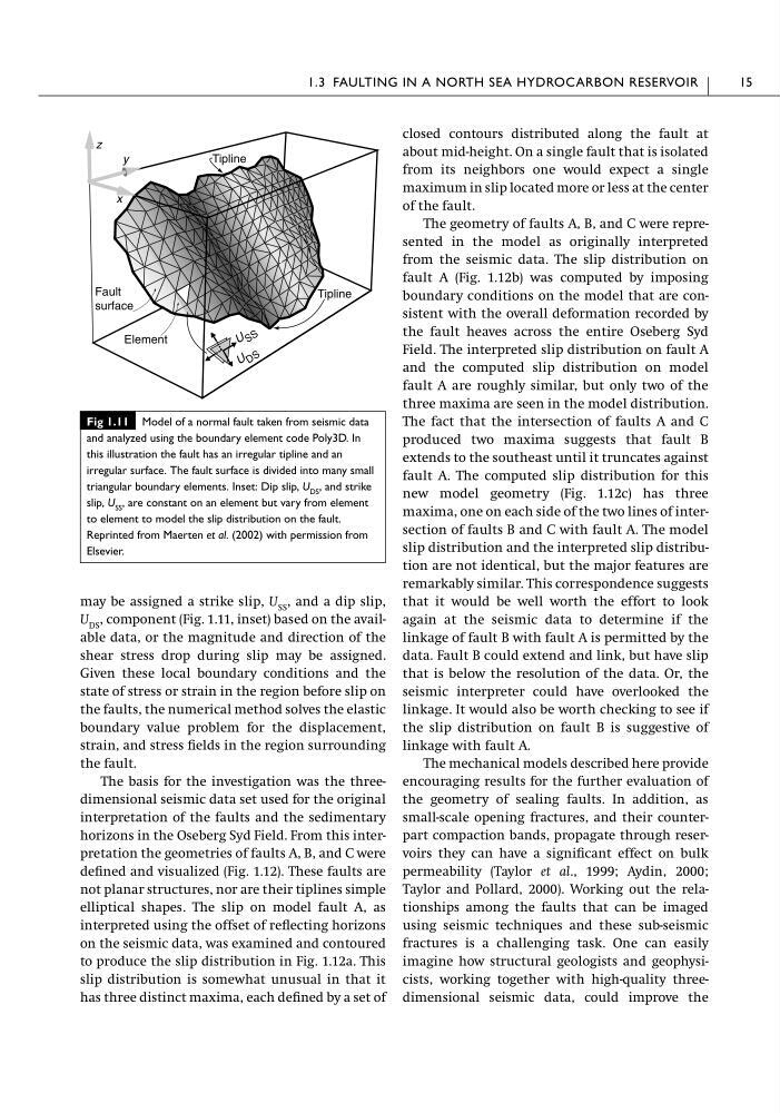
may be assigned a strike slip, U SS , and a dip slip,
U DS , component (Fig. 1.11, inset) based on the available data, or the magnitude and direction of the
shear stress drop during slip may be assigned.
Given these local boundary conditions and the
state of stress or strain in the region before slip on
the faults, the numerical method solves the elastic
boundary value problem for the displacement,
strain, and stress fields in the region surrounding
the fault.
The basis for the investigation was the threedimensional seismic data set used for the original
interpretation of the faults and the sedimentary
horizons in the Oseberg Syd Field. From this interpretation the geometries of faults A, B, and C were
defined and visualized (Fig. 1.12). These faults are
not planar structures, nor are their tiplines simple
elliptical shapes. The slip on model fault A, as
interpreted using the offset of reflecting horizons
on the seismic data, was examined and contoured
to produce the slip distribution in Fig. 1.12a. This
slip distribution is somewhat unusual in that it
has three distinct maxima, each defined by a set of
closed contours distributed along the fault at
about mid-height. On a single fault that is isolated
from its neighbors one would expect a single
maximum in slip located more or less at the center
of the fault.
The geometry of faults A, B, and C were represented in the model as originally interpreted
from the seismic data. The slip distribution on
fault A (Fig. 1.12b) was computed by imposing
boundary conditions on the model that are consistent with the overall deformation recorded by
the fault heaves across the entire Oseberg Syd
Field. The interpreted slip distribution on fault A
and the computed slip distribution on model
fault A are roughly similar, but only two of the
three maxima are seen in the model distribution.
The fact that the intersection of faults A and C
produced two maxima suggests that fault B
extends to the southeast until it truncates against
fault A. The computed slip distribution for this
new model geometry (Fig. 1.12c) has three
maxima, one on each side of the two lines of intersection of faults B and C with fault A. The model
slip distribution and the interpreted slip distribution are not identical, but the major features are
remarkably similar. This correspondence suggests
that it would be well worth the effort to look
again at the seismic data to determine if the
linkage of fault B with fault A is permitted by the
data. Fault B could extend and link, but have slip
that is below the resolution of the data. Or, the
seismic interpreter could have overlooked the
linkage. It would also be worth checking to see if
the slip distribution on fault B is suggestive of
linkage with fault A.
The mechanical models described here provide
encouraging results for the further evaluation of
the geometry of sealing faults. In addition, as
small-scale opening fractures, and their counterpart compaction bands, propagate through reservoirs they can have a significant effect on bulk
permeability (Taylor et al., 1999; Aydin, 2000;
Taylor and Pollard, 2000). Working out the relationships among the faults that can be imaged
using seismic techniques and these sub-seismic
fractures is a challenging task. One can easily
imagine how structural geologists and geophysicists, working together with high-quality threedimensional seismic data, could improve the
1.3 FAULTING IN A NORTH SEA HYDROCARBON RESERVOIR
15
Element
Tipline
x
y
z
Tipline
U S S
U D S
Fault
surface
Fig 1.11 Model of a normal fault taken from seismic data
and analyzed using the boundary element code Poly3D. In
this illustration the fault has an irregular tipline and an
irregular surface. The fault surface is divided into many small
triangular boundary elements. Inset: Dip slip, U DS , and strike
slip, U SS , are constant on an element but vary from element
to element to model the slip distribution on the fault.
Reprinted from Maerten et al. (2002) with permission from
Elsevier.
U DS , component (Fig. 1.11, inset) based on the available data, or the magnitude and direction of the
shear stress drop during slip may be assigned.
Given these local boundary conditions and the
state of stress or strain in the region before slip on
the faults, the numerical method solves the elastic
boundary value problem for the displacement,
strain, and stress fields in the region surrounding
the fault.
The basis for the investigation was the threedimensional seismic data set used for the original
interpretation of the faults and the sedimentary
horizons in the Oseberg Syd Field. From this interpretation the geometries of faults A, B, and C were
defined and visualized (Fig. 1.12). These faults are
not planar structures, nor are their tiplines simple
elliptical shapes. The slip on model fault A, as
interpreted using the offset of reflecting horizons
on the seismic data, was examined and contoured
to produce the slip distribution in Fig. 1.12a. This
slip distribution is somewhat unusual in that it
has three distinct maxima, each defined by a set of
closed contours distributed along the fault at
about mid-height. On a single fault that is isolated
from its neighbors one would expect a single
maximum in slip located more or less at the center
of the fault.
The geometry of faults A, B, and C were represented in the model as originally interpreted
from the seismic data. The slip distribution on
fault A (Fig. 1.12b) was computed by imposing
boundary conditions on the model that are consistent with the overall deformation recorded by
the fault heaves across the entire Oseberg Syd
Field. The interpreted slip distribution on fault A
and the computed slip distribution on model
fault A are roughly similar, but only two of the
three maxima are seen in the model distribution.
The fact that the intersection of faults A and C
produced two maxima suggests that fault B
extends to the southeast until it truncates against
fault A. The computed slip distribution for this
new model geometry (Fig. 1.12c) has three
maxima, one on each side of the two lines of intersection of faults B and C with fault A. The model
slip distribution and the interpreted slip distribution are not identical, but the major features are
remarkably similar. This correspondence suggests
that it would be well worth the effort to look
again at the seismic data to determine if the
linkage of fault B with fault A is permitted by the
data. Fault B could extend and link, but have slip
that is below the resolution of the data. Or, the
seismic interpreter could have overlooked the
linkage. It would also be worth checking to see if
the slip distribution on fault B is suggestive of
linkage with fault A.
The mechanical models described here provide
encouraging results for the further evaluation of
the geometry of sealing faults. In addition, as
small-scale opening fractures, and their counterpart compaction bands, propagate through reservoirs they can have a significant effect on bulk
permeability (Taylor et al., 1999; Aydin, 2000;
Taylor and Pollard, 2000). Working out the relationships among the faults that can be imaged
using seismic techniques and these sub-seismic
fractures is a challenging task. One can easily
imagine how structural geologists and geophysicists, working together with high-quality threedimensional seismic data, could improve the
1.3 FAULTING IN A NORTH SEA HYDROCARBON RESERVOIR
15
Element
Tipline
x
y
z
Tipline
U S S
U D S
Fault
surface
Fig 1.11 Model of a normal fault taken from seismic data
and analyzed using the boundary element code Poly3D. In
this illustration the fault has an irregular tipline and an
irregular surface. The fault surface is divided into many small
triangular boundary elements. Inset: Dip slip, U DS , and strike
slip, U SS , are constant on an element but vary from element
to element to model the slip distribution on the fault.
Reprinted from Maerten et al. (2002) with permission from
Elsevier.