

a given particle along its path, while the latter
describes the velocity of all particles that pass
through a given location.
The time derivative of the local velocity (7.60)
at a given current location is:
(7.61)
The quantity defined in (7.61) is referred to as the
local rate of change of velocity (Malvern, 1969) and
not as the acceleration because it does not necessarily define the particle acceleration (7.59) at the
position x and time t. To appreciate this apparent
contradiction recall the velocity distribution
(5.19) within a rising viscous sphere (Fig. 5.12).
This is an example of steady flow, which means that
all of the kinematic quantities are constant in
time at every point. Thus, at every current position x the time derivative of velocity as defined in
(7.61) is identically zero. On the other hand the
Ѩv
Ѩt | x
ϭ
Ѩ
Ѩt
g(x, t)
velocity of a given particle that follows one of the
stream lines illustrated in Fig. 5.12b changes with
position, being greater where the stream lines are
more closely spaced. This particle and every other
particle, except those at the stagnation points at
the top and bottom of the sphere, accelerate and
decelerate as they circulate within the sphere.
Clearly one cannot take the local rate of change of
velocity (7.61) as the particle acceleration (7.59) in
this particular case.
It is important to clarify the general relationship between the particle acceleration (7.59) and
the local rate of change of velocity (7.61). We do
this by showing how to calculate the material
time derivative of a quantity given a spatial
description of the kinematics of that quantity
(Malvern, 1969). We start with the function g(x, t)
that describes the local velocity (7.60). The underlying premise is that particle motion may be
defined by a function x(X, t) for the referential
description of motion (7.57). This relationship is
substituted for the spatial coordinates, x, in the
function for the local velocity to transform it to a
function of the material coordinates X:
(7.62)
Because we have started with a spatial description
of motion the referential description given by the
function x ϭ x(X, t) may not be known, but knowledge of this function is not necessary to define the
material time derivative of (7.62). Recalling the
Chain Rule of calculus, if z ϭ f(x, y) but x ϭ x(r, s)
and yϭy(r, s) one takes the partial derivative of z
with respect to s holding r constant as (Varberg
and Purcell, 1992):
(7.63)
Making the appropriate associations for the quantities in the vector function (7.62) we have:
(7.64)
The left-hand side is the material time derivative
of the velocity which is, by (7.59), the particle
acceleration, a. The first partial derivative on the
right-hand side may be calculated from the local
velocity (7.60), which is given. The second partial
derivative is the particle velocity (7.58), but that is
equivalent to the local velocity, v, defined in (7.60).
Ѩv
Ѩt | X
ϭ
Ѩv
Ѩx |
t
Ѩx
Ѩt | X
ϩ
Ѩv
Ѩt | x
Ѩt
Ѩt | X
Ѩz
Ѩs |
r
ϭ
Ѩz
Ѩx |
y
Ѩx
Ѩs |
r
ϩ
Ѩz
Ѩy |
x
Ѩy
Ѩs |
r
v ϭ g[x(X, t), t] ϵ G(X, t)
7.3 THE DEFORMABLE CONTINUUM
265
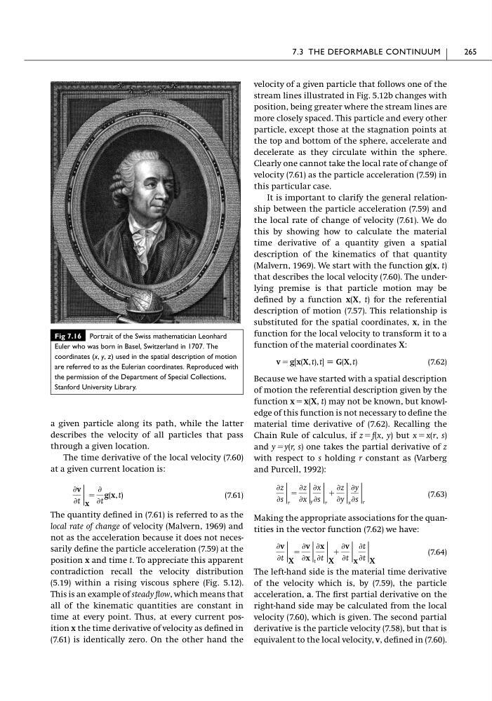
Fig 7.16 Portrait of the Swiss mathematician Leonhard
Euler who was born in Basel, Switzerland in 1707. The
coordinates (x, y, z) used in the spatial description of motion
are referred to as the Eulerian coordinates. Reproduced with
the permission of the Department of Special Collections,
Stanford University Library.
describes the velocity of all particles that pass
through a given location.
The time derivative of the local velocity (7.60)
at a given current location is:
(7.61)
The quantity defined in (7.61) is referred to as the
local rate of change of velocity (Malvern, 1969) and
not as the acceleration because it does not necessarily define the particle acceleration (7.59) at the
position x and time t. To appreciate this apparent
contradiction recall the velocity distribution
(5.19) within a rising viscous sphere (Fig. 5.12).
This is an example of steady flow, which means that
all of the kinematic quantities are constant in
time at every point. Thus, at every current position x the time derivative of velocity as defined in
(7.61) is identically zero. On the other hand the
Ѩv
Ѩt | x
ϭ
Ѩ
Ѩt
g(x, t)
velocity of a given particle that follows one of the
stream lines illustrated in Fig. 5.12b changes with
position, being greater where the stream lines are
more closely spaced. This particle and every other
particle, except those at the stagnation points at
the top and bottom of the sphere, accelerate and
decelerate as they circulate within the sphere.
Clearly one cannot take the local rate of change of
velocity (7.61) as the particle acceleration (7.59) in
this particular case.
It is important to clarify the general relationship between the particle acceleration (7.59) and
the local rate of change of velocity (7.61). We do
this by showing how to calculate the material
time derivative of a quantity given a spatial
description of the kinematics of that quantity
(Malvern, 1969). We start with the function g(x, t)
that describes the local velocity (7.60). The underlying premise is that particle motion may be
defined by a function x(X, t) for the referential
description of motion (7.57). This relationship is
substituted for the spatial coordinates, x, in the
function for the local velocity to transform it to a
function of the material coordinates X:
(7.62)
Because we have started with a spatial description
of motion the referential description given by the
function x ϭ x(X, t) may not be known, but knowledge of this function is not necessary to define the
material time derivative of (7.62). Recalling the
Chain Rule of calculus, if z ϭ f(x, y) but x ϭ x(r, s)
and yϭy(r, s) one takes the partial derivative of z
with respect to s holding r constant as (Varberg
and Purcell, 1992):
(7.63)
Making the appropriate associations for the quantities in the vector function (7.62) we have:
(7.64)
The left-hand side is the material time derivative
of the velocity which is, by (7.59), the particle
acceleration, a. The first partial derivative on the
right-hand side may be calculated from the local
velocity (7.60), which is given. The second partial
derivative is the particle velocity (7.58), but that is
equivalent to the local velocity, v, defined in (7.60).
Ѩv
Ѩt | X
ϭ
Ѩv
Ѩx |
t
Ѩx
Ѩt | X
ϩ
Ѩv
Ѩt | x
Ѩt
Ѩt | X
Ѩz
Ѩs |
r
ϭ
Ѩz
Ѩx |
y
Ѩx
Ѩs |
r
ϩ
Ѩz
Ѩy |
x
Ѩy
Ѩs |
r
v ϭ g[x(X, t), t] ϵ G(X, t)
7.3 THE DEFORMABLE CONTINUUM
265
Fig 7.16 Portrait of the Swiss mathematician Leonhard
Euler who was born in Basel, Switzerland in 1707. The
coordinates (x, y, z) used in the spatial description of motion
are referred to as the Eulerian coordinates. Reproduced with
the permission of the Department of Special Collections,
Stanford University Library.