

the mechanisms of faulting may change with
depth as temperature and pressure increase, such
that brittle fracture and friction dominate at
shallow depths and ductile flow dominates at
greater depths. In this conceptual model the resistance to shearing increases with depth to this
transition and then decreases with depth. In a vertical section viewed perpendicular to the fault
(A–AЈ), dynamic shearing begins at depth, near
the brittle–ductile transition and spreads out over
the fault surface at a velocity of about 3 km s
Ϫ1 ,
eventually reaching the Earth’s surface.
The Imperial Valley earthquake is noteworthy
because it occurred within a dense array of geodetic and geophysical instruments and there were
abundant cultural features for the geologists to
measure at the surface (Savage et al., 1979). The
mechanical model reviewed here was constructed
using data from the seismographs and strong
motion instruments that monitored this event
(Archuleta, 1984). The results are not unique and
the choice of model parameters could be debated,
but that is not the issue here. This model provides
an excellent example of the insight one can gain
about phenomena that are otherwise totally inaccessible to direct observation.
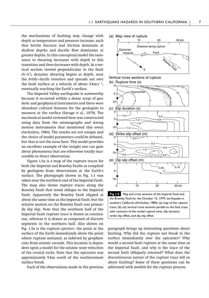
Figure 1.5a is a map of the rupture traces for
both the Imperial and Brawley Faults as compiled
by geologists from observations at the Earth’s
surface. The photograph shown in Fig. 1.1 was
taken near the northern end of the Imperial Fault.
The map also shows rupture traces along the
Brawley Fault that trend oblique to the Imperial
Fault. Apparently the Brawley Fault slipped at
about the same time as the Imperial Fault, but the
relative motion on the Brawley Fault was primarily dip slip. Note that the southern half of the
Imperial Fault rupture trace is drawn as continuous, whereas it is drawn as composed of discrete
segments in the northern half. Also shown on
Fig. 1.5a is the rupture epicenter, the point at the
surface of the Earth immediately above the point
where rupture initiated, as inferred by geophysicists from seismic records. This location is dependent upon a model for the seismic wave velocities
of the crustal rocks. Note that the epicenter was
approximately 5 km south of the southernmost
surface break.
Each of the observations made in the previous
paragraph brings up interesting questions about
faulting. Why did the rupture not break to the
surface immediately over the epicenter? Why
would a second fault rupture at the same time as
the Imperial Fault, and why is the trace of the
second fault obliquely oriented? What does the
discontinuous nature of the rupture trace tell us
about faulting? Some of these questions can be
addressed with models for the rupture process.
1.1 EARTHQUAKE HAZARDS IN SOUTHERN CALIFORNIA
7
Distance along rupture
0
10
20
30 km
12
10
8
6
B r a w le y F a u lt
N
Imperial
Fault
(a) Map view of rupture
(b) Rupture time (s)
(c) Slip duration (s)
(d) Strike slip offset (m)
(e) Dip slip offset (m)
0
10
20
30 km
10
5
0
10
5
0
10
5
0
10
5
0
2
0.8
0.4
1.6
0.4
1.2
1.2
4
0.2
0.2
1.0
0.6
0.6
0.6
1.0
1.0
1.4
0.08
0.16
0
Epicenter
Hypocenter
Vertical cross sections of rupture
Fig 1.5 Map and cross sections of the Imperial Fault and
the Brawley Fault for the October 15, 1979, earthquake in
southern California (Archuleta, 1984): (a) map of the rupture
trace; (b)–(e) vertical cross sections parallel to the fault trace
with contours of the model rupture time, slip duration,
strike slip offset, and dip slip offset.
depth as temperature and pressure increase, such
that brittle fracture and friction dominate at
shallow depths and ductile flow dominates at
greater depths. In this conceptual model the resistance to shearing increases with depth to this
transition and then decreases with depth. In a vertical section viewed perpendicular to the fault
(A–AЈ), dynamic shearing begins at depth, near
the brittle–ductile transition and spreads out over
the fault surface at a velocity of about 3 km s
Ϫ1 ,
eventually reaching the Earth’s surface.
The Imperial Valley earthquake is noteworthy
because it occurred within a dense array of geodetic and geophysical instruments and there were
abundant cultural features for the geologists to
measure at the surface (Savage et al., 1979). The
mechanical model reviewed here was constructed
using data from the seismographs and strong
motion instruments that monitored this event
(Archuleta, 1984). The results are not unique and
the choice of model parameters could be debated,
but that is not the issue here. This model provides
an excellent example of the insight one can gain
about phenomena that are otherwise totally inaccessible to direct observation.
Figure 1.5a is a map of the rupture traces for
both the Imperial and Brawley Faults as compiled
by geologists from observations at the Earth’s
surface. The photograph shown in Fig. 1.1 was
taken near the northern end of the Imperial Fault.
The map also shows rupture traces along the
Brawley Fault that trend oblique to the Imperial
Fault. Apparently the Brawley Fault slipped at
about the same time as the Imperial Fault, but the
relative motion on the Brawley Fault was primarily dip slip. Note that the southern half of the
Imperial Fault rupture trace is drawn as continuous, whereas it is drawn as composed of discrete
segments in the northern half. Also shown on
Fig. 1.5a is the rupture epicenter, the point at the
surface of the Earth immediately above the point
where rupture initiated, as inferred by geophysicists from seismic records. This location is dependent upon a model for the seismic wave velocities
of the crustal rocks. Note that the epicenter was
approximately 5 km south of the southernmost
surface break.
Each of the observations made in the previous
paragraph brings up interesting questions about
faulting. Why did the rupture not break to the
surface immediately over the epicenter? Why
would a second fault rupture at the same time as
the Imperial Fault, and why is the trace of the
second fault obliquely oriented? What does the
discontinuous nature of the rupture trace tell us
about faulting? Some of these questions can be
addressed with models for the rupture process.
1.1 EARTHQUAKE HAZARDS IN SOUTHERN CALIFORNIA
7
Distance along rupture
0
10
20
30 km
12
10
8
6
B r a w le y F a u lt
N
Imperial
Fault
(a) Map view of rupture
(b) Rupture time (s)
(c) Slip duration (s)
(d) Strike slip offset (m)
(e) Dip slip offset (m)
0
10
20
30 km
10
5
0
10
5
0
10
5
0
10
5
0
2
0.8
0.4
1.6
0.4
1.2
1.2
4
0.2
0.2
1.0
0.6
0.6
0.6
1.0
1.0
1.4
0.08
0.16
0
Epicenter
Hypocenter
Vertical cross sections of rupture
Fig 1.5 Map and cross sections of the Imperial Fault and
the Brawley Fault for the October 15, 1979, earthquake in
southern California (Archuleta, 1984): (a) map of the rupture
trace; (b)–(e) vertical cross sections parallel to the fault trace
with contours of the model rupture time, slip duration,
strike slip offset, and dip slip offset.