

rather than 0, so quantities such as these can be
included in the algebraic manipulation of dimensional equations (Obert and Duvall, 1967).
Similarly, the symbol 1 is used for dimensionless
constants such as .
Dimensional analysis provides a procedure to
evaluate equations involving physical quantities:
those purporting to describe some physical object,
event, or process. This procedure enables one to
check whether an equation might be in error by
being dimensionally inconsistent. This is probably
the first thing you should do when confronted
with an unfamiliar equation, especially a very
complicated one. For example, suppose that you
are reading the geological literature and you come
across the following equation for the change in
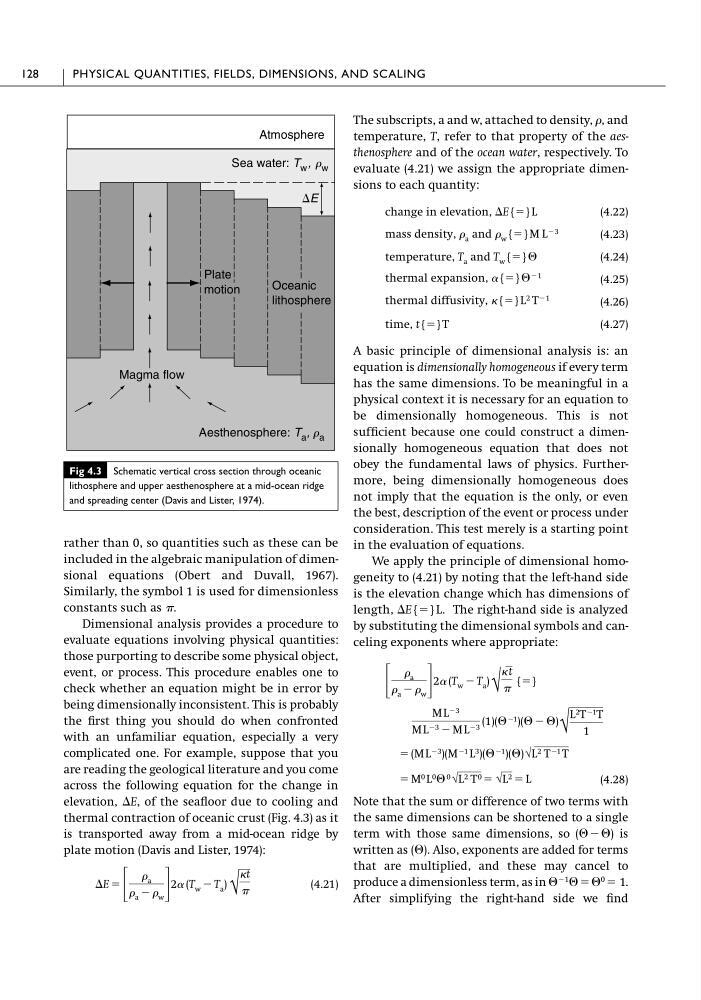
elevation, ⌬E, of the seafloor due to cooling and
thermal contraction of oceanic crust (Fig. 4.3) as it
is transported away from a mid-ocean ridge by
plate motion (Davis and Lister, 1974):
(4.21)
⌬E ϭ
΄
a
a Ϫ w ΅
2␣ (T w Ϫ T a )
√
t
The subscripts, a and w, attached to density, , and
temperature, T, refer to that property of the aesthenosphere and of the ocean water, respectively. To
evaluate (4.21) we assign the appropriate dimensions to each quantity:
(4.22)
(4.23)
(4.24)
(4.25)
(4.26)
(4.27)
A basic principle of dimensional analysis is: an
equation is dimensionally homogeneous if every term
has the same dimensions. To be meaningful in a
physical context it is necessary for an equation to
be dimensionally homogeneous. This is not
sufficient because one could construct a dimensionally homogeneous equation that does not
obey the fundamental laws of physics. Furthermore, being dimensionally homogeneous does
not imply that the equation is the only, or even
the best, description of the event or process under
consideration. This test merely is a starting point
in the evaluation of equations.
We apply the principle of dimensional homogeneity to (4.21) by noting that the left-hand side
is the elevation change which has dimensions of
length,
The right-hand side is analyzed
by substituting the dimensional symbols and canceling exponents where appropriate:
(4.28)
Note that the sum or difference of two terms with
the same dimensions can be shortened to a single
term with those same dimensions, so (⌰Ϫ⌰) is
written as (⌰). Also, exponents are added for terms
that are multiplied, and these may cancel to
produce a dimensionless term, as in ⌰
Ϫ1 ⌰ϭ⌰
0 ϭ 1.
After simplifying the right-hand side we find
ϭ M 0 L 0 ⌰ 0 √L 2 T 0 ϭ √L 2 ϭ L
ϭ (M L Ϫ3 )(M Ϫ1 L 3 )(⌰ Ϫ1 )(⌰) √L 2 T Ϫ1 T
M L Ϫ3
M L Ϫ3 Ϫ M L Ϫ3 (1)(⌰ Ϫ1 )(⌰ Ϫ ⌰)
√
L 2 T Ϫ1 T
1
΄
a
a Ϫ w ΅ 2␣ (T w Ϫ T a ) √
t
{ϭ}
⌬E{ϭ}L.
time, t{ϭ}T
thermal diffusivity, {ϭ}L 2 T Ϫ1
thermal expansion, ␣{ϭ}⌰ Ϫ1
temperature, T a and T w {ϭ}⌰
mass density, a and w {ϭ}M L Ϫ3
change in elevation, ⌬E{ϭ}L
128
PHYSICAL QUANTITIES, FIELDS, DIMENSIONS, AND SCALING
Fig 4.3 Schematic vertical cross section through oceanic
lithosphere and upper aesthenosphere at a mid-ocean ridge
and spreading center (Davis and Lister, 1974).
seawater
Atmosphere
Sea water: T w , r w
Plate
motion
Oceanic
lithosphere
Magma flow
Aesthenosphere: T a , r a
⌬E
included in the algebraic manipulation of dimensional equations (Obert and Duvall, 1967).
Similarly, the symbol 1 is used for dimensionless
constants such as .
Dimensional analysis provides a procedure to
evaluate equations involving physical quantities:
those purporting to describe some physical object,
event, or process. This procedure enables one to
check whether an equation might be in error by
being dimensionally inconsistent. This is probably
the first thing you should do when confronted
with an unfamiliar equation, especially a very
complicated one. For example, suppose that you
are reading the geological literature and you come
across the following equation for the change in
elevation, ⌬E, of the seafloor due to cooling and
thermal contraction of oceanic crust (Fig. 4.3) as it
is transported away from a mid-ocean ridge by
plate motion (Davis and Lister, 1974):
(4.21)
⌬E ϭ
΄
a
a Ϫ w ΅
2␣ (T w Ϫ T a )
√
t
The subscripts, a and w, attached to density, , and
temperature, T, refer to that property of the aesthenosphere and of the ocean water, respectively. To
evaluate (4.21) we assign the appropriate dimensions to each quantity:
(4.22)
(4.23)
(4.24)
(4.25)
(4.26)
(4.27)
A basic principle of dimensional analysis is: an
equation is dimensionally homogeneous if every term
has the same dimensions. To be meaningful in a
physical context it is necessary for an equation to
be dimensionally homogeneous. This is not
sufficient because one could construct a dimensionally homogeneous equation that does not
obey the fundamental laws of physics. Furthermore, being dimensionally homogeneous does
not imply that the equation is the only, or even
the best, description of the event or process under
consideration. This test merely is a starting point
in the evaluation of equations.
We apply the principle of dimensional homogeneity to (4.21) by noting that the left-hand side
is the elevation change which has dimensions of
length,
The right-hand side is analyzed
by substituting the dimensional symbols and canceling exponents where appropriate:
(4.28)
Note that the sum or difference of two terms with
the same dimensions can be shortened to a single
term with those same dimensions, so (⌰Ϫ⌰) is
written as (⌰). Also, exponents are added for terms
that are multiplied, and these may cancel to
produce a dimensionless term, as in ⌰
Ϫ1 ⌰ϭ⌰
0 ϭ 1.
After simplifying the right-hand side we find
ϭ M 0 L 0 ⌰ 0 √L 2 T 0 ϭ √L 2 ϭ L
ϭ (M L Ϫ3 )(M Ϫ1 L 3 )(⌰ Ϫ1 )(⌰) √L 2 T Ϫ1 T
M L Ϫ3
M L Ϫ3 Ϫ M L Ϫ3 (1)(⌰ Ϫ1 )(⌰ Ϫ ⌰)
√
L 2 T Ϫ1 T
1
΄
a
a Ϫ w ΅ 2␣ (T w Ϫ T a ) √
t
{ϭ}
⌬E{ϭ}L.
time, t{ϭ}T
thermal diffusivity, {ϭ}L 2 T Ϫ1
thermal expansion, ␣{ϭ}⌰ Ϫ1
temperature, T a and T w {ϭ}⌰
mass density, a and w {ϭ}M L Ϫ3
change in elevation, ⌬E{ϭ}L
128
PHYSICAL QUANTITIES, FIELDS, DIMENSIONS, AND SCALING
Fig 4.3 Schematic vertical cross section through oceanic
lithosphere and upper aesthenosphere at a mid-ocean ridge
and spreading center (Davis and Lister, 1974).
seawater
Atmosphere
Sea water: T w , r w
Plate
motion
Oceanic
lithosphere
Magma flow
Aesthenosphere: T a , r a
⌬E