

point. This can, however, present conceptual difficulties. For example, consider the mass density, ,
of a sample of rock as determined by:
(4.8)
Here ␦M is the mass and ␦V is the volume of the
sample. Mass is equivalent to weight divided by
the known acceleration of gravity and it is a
straightforward matter to weigh the sample. If
the sample is cylindrical the volume is readily calculated after measuring the height and diameter.
With these numbers in hand, (4.8) is used to calculate the mass density of the sample. Suppose
we decide to use this density as representative of
the rock mass under consideration. Plotting
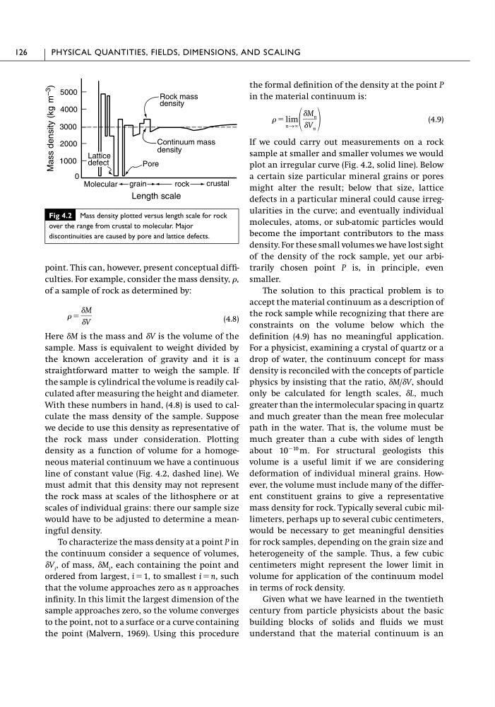
density as a function of volume for a homogeneous material continuum we have a continuous
line of constant value (Fig. 4.2, dashed line). We
must admit that this density may not represent
the rock mass at scales of the lithosphere or at
scales of individual grains: there our sample size
would have to be adjusted to determine a meaningful density.
To characterize the mass density at a point P in
the continuum consider a sequence of volumes,
␦V i , of mass, ␦M i , each containing the point and
ordered from largest, i ϭ 1, to smallest i ϭ n, such
that the volume approaches zero as n approaches
infinity. In this limit the largest dimension of the
sample approaches zero, so the volume converges
to the point, not to a surface or a curve containing
the point (Malvern, 1969). Using this procedure
ϭ
␦M
␦V
the formal definition of the density at the point P
in the material continuum is:
(4.9)
If we could carry out measurements on a rock
sample at smaller and smaller volumes we would
plot an irregular curve (Fig. 4.2, solid line). Below
a certain size particular mineral grains or pores
might alter the result; below that size, lattice
defects in a particular mineral could cause irregularities in the curve; and eventually individual
molecules, atoms, or sub-atomic particles would
become the important contributors to the mass
density. For these small volumes we have lost sight
of the density of the rock sample, yet our arbitrarily chosen point P is, in principle, even
smaller.
The solution to this practical problem is to
accept the material continuum as a description of
the rock sample while recognizing that there are
constraints on the volume below which the
definition (4.9) has no meaningful application.
For a physicist, examining a crystal of quartz or a
drop of water, the continuum concept for mass
density is reconciled with the concepts of particle
physics by insisting that the ratio, ␦M/␦V, should
only be calculated for length scales, ␦L, much
greater than the intermolecular spacing in quartz
and much greater than the mean free molecular
path in the water. That is, the volume must be
much greater than a cube with sides of length
about 10
Ϫ10 m. For structural geologists this
volume is a useful limit if we are considering
deformation of individual mineral grains. However, the volume must include many of the different constituent grains to give a representative
mass density for rock. Typically several cubic millimeters, perhaps up to several cubic centimeters,
would be necessary to get meaningful densities
for rock samples, depending on the grain size and
heterogeneity of the sample. Thus, a few cubic
centimeters might represent the lower limit in
volume for application of the continuum model
in terms of rock density.
Given what we have learned in the twentieth
century from particle physicists about the basic
building blocks of solids and fluids we must
understand that the material continuum is an
ϭ lim
n→ϱ
␦M n
␦V n
126
PHYSICAL QUANTITIES, FIELDS, DIMENSIONS, AND SCALING
Pore
Length scale
0
1000
2000
3000
4000
5000
Lattice
defect
Molecular
grain
rock
crustal
Continuum mass
density
Rock mass
density
Mass density (kg m –3
)
Fig 4.2 Mass density plotted versus length scale for rock
over the range from crustal to molecular. Major
discontinuities are caused by pore and lattice defects.
of a sample of rock as determined by:
(4.8)
Here ␦M is the mass and ␦V is the volume of the
sample. Mass is equivalent to weight divided by
the known acceleration of gravity and it is a
straightforward matter to weigh the sample. If
the sample is cylindrical the volume is readily calculated after measuring the height and diameter.
With these numbers in hand, (4.8) is used to calculate the mass density of the sample. Suppose
we decide to use this density as representative of
the rock mass under consideration. Plotting
density as a function of volume for a homogeneous material continuum we have a continuous
line of constant value (Fig. 4.2, dashed line). We
must admit that this density may not represent
the rock mass at scales of the lithosphere or at
scales of individual grains: there our sample size
would have to be adjusted to determine a meaningful density.
To characterize the mass density at a point P in
the continuum consider a sequence of volumes,
␦V i , of mass, ␦M i , each containing the point and
ordered from largest, i ϭ 1, to smallest i ϭ n, such
that the volume approaches zero as n approaches
infinity. In this limit the largest dimension of the
sample approaches zero, so the volume converges
to the point, not to a surface or a curve containing
the point (Malvern, 1969). Using this procedure
ϭ
␦M
␦V
the formal definition of the density at the point P
in the material continuum is:
(4.9)
If we could carry out measurements on a rock
sample at smaller and smaller volumes we would
plot an irregular curve (Fig. 4.2, solid line). Below
a certain size particular mineral grains or pores
might alter the result; below that size, lattice
defects in a particular mineral could cause irregularities in the curve; and eventually individual
molecules, atoms, or sub-atomic particles would
become the important contributors to the mass
density. For these small volumes we have lost sight
of the density of the rock sample, yet our arbitrarily chosen point P is, in principle, even
smaller.
The solution to this practical problem is to
accept the material continuum as a description of
the rock sample while recognizing that there are
constraints on the volume below which the
definition (4.9) has no meaningful application.
For a physicist, examining a crystal of quartz or a
drop of water, the continuum concept for mass
density is reconciled with the concepts of particle
physics by insisting that the ratio, ␦M/␦V, should
only be calculated for length scales, ␦L, much
greater than the intermolecular spacing in quartz
and much greater than the mean free molecular
path in the water. That is, the volume must be
much greater than a cube with sides of length
about 10
Ϫ10 m. For structural geologists this
volume is a useful limit if we are considering
deformation of individual mineral grains. However, the volume must include many of the different constituent grains to give a representative
mass density for rock. Typically several cubic millimeters, perhaps up to several cubic centimeters,
would be necessary to get meaningful densities
for rock samples, depending on the grain size and
heterogeneity of the sample. Thus, a few cubic
centimeters might represent the lower limit in
volume for application of the continuum model
in terms of rock density.
Given what we have learned in the twentieth
century from particle physicists about the basic
building blocks of solids and fluids we must
understand that the material continuum is an
ϭ lim
n→ϱ
␦M n
␦V n
126
PHYSICAL QUANTITIES, FIELDS, DIMENSIONS, AND SCALING
Pore
Length scale
0
1000
2000
3000
4000
5000
Lattice
defect
Molecular
grain
rock
crustal
Continuum mass
density
Rock mass
density
Mass density (kg m –3
)
Fig 4.2 Mass density plotted versus length scale for rock
over the range from crustal to molecular. Major
discontinuities are caused by pore and lattice defects.