

Dividing each term of (3.128) by the first term
in parentheses we have:
(3.130)
The first constant, m , is the average of the two
principal normal curvatures and is referred to as
the mean principal normal curvature:
(3.131)
The second constant, g , is the product of the principal curvatures and is called the Gaussian curvature:
(3.132)
For example, the mean curvature for the helicoidal surface is found by substituting the
coefficients of the fundamental forms, (3.96) and
(3.112), into (3.131) to find
. The fact that the
mean normal curvature is zero is consistent with
the two principal curvatures being equal and
opposite in sign. Surfaces that satisfy the condition of zero mean curvature are called minimal surfaces. The Gaussian curvature for the helicoidal
surface is found by substituting (3.96) and (3.112)
into (3.132) to find
. The Gaussian
curvature is not a function of the parameter v and
therefore is constant along a given v-parameter
g ϭ Ϫc
2 ր(c
2 ϩ u
2 )
2
m ϭ 0
g ϭ
(LN Ϫ M
2 )
(EG Ϫ F
2 )
ϭ 1 2
m ϭ
(EN Ϫ 2FM ϩ GL)
2(EG Ϫ F
2
)
ϭ
1
2
( 1 ϩ 2 )
ϩ g ϭ 0
2
o
Ϫ 2 m o
circular helix. Along the mid-line of the helicoidal
surface, u ϭ 0, the Gaussian curvature is a constant equal to the negative of the squared rate of
twist.
We have identified the three possible nonplanar shapes (hyperbolic, parabolic, and elliptic)
in the vicinity of a particular point on a surface
based on the sign of the numerator in (3.132) and
these shapes are illustrated in Fig. 3.29. Because
the denominator in (3.132) always is positive, the
sign of the Gaussian curvature is determined by
the numerator. Thus the sign of g may be used to
distinguish these three non-planar shapes. Taken
together, the signs of the Gaussian and the mean
curvature may be used to categorize surfaces with
respect to orientation in keeping with geological
conventions (Roberts, 2001). Consider the Monge
patch (3.58) with the (x, y)-plane horizontal and
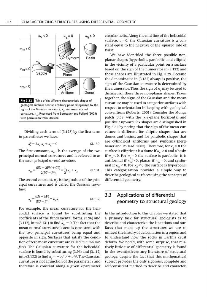
positive z upward. Six shapes are distinguished in
Fig. 3.32 by noting that the sign of the mean curvature is different for elliptic shapes that are
domes and basins, and for parabolic shapes that
are cylindrical antiforms and synforms (Bergbauer and Pollard, 2003). Therefore, for g Ͼ 0 the
surface is elliptic; it is a dome if m Ͼ 0 and a basin
if m Ͻ 0. For g ϭ 0 the surface is parabolic; it is
antiformal if m Ͼ 0, planar if m ϭ 0, and synformal if m Ͻ 0. For g Ͻ 0 the surface is hyperbolic.
This categorization provides a simple way to
describe geological surfaces using the concepts of
differential geometry.
3.3 Applications of differential
geometry to structural geology
In the introduction to this chapter we stated that
a primary task for structural geologists is to
describe and characterize the lineations and surfaces that make up the structures we use to
unravel the history of deformation in a region and
to understand how the rocks in Earth’s crust
deform. We noted, with some surprise, that relatively little use of differential geometry is found
in the twentieth-century literature of structural
geology, despite the fact that this mathematical
subject provides the only rigorous, complete and
self-consistent method to describe and character114
CHARACTERIZING STRUCTURES USING DIFFERENTIAL GEOMETRY
Fig 3.32 Table of six different characteristic shapes of
geological surfaces near an arbitrary point categorized by the
signs of the Gaussian curvature, g , and mean normal
curvature, m . Reprinted from Bergbauer and Pollard (2003)
with permission from Elsevier.
K g < 0
K g > 0
K g = 0
K m = 0
K m > 0
K m < 0
Plane
Antiform
Synform
Saddle
Basin
Dome
in parentheses we have:
(3.130)
The first constant, m , is the average of the two
principal normal curvatures and is referred to as
the mean principal normal curvature:
(3.131)
The second constant, g , is the product of the principal curvatures and is called the Gaussian curvature:
(3.132)
For example, the mean curvature for the helicoidal surface is found by substituting the
coefficients of the fundamental forms, (3.96) and
(3.112), into (3.131) to find
. The fact that the
mean normal curvature is zero is consistent with
the two principal curvatures being equal and
opposite in sign. Surfaces that satisfy the condition of zero mean curvature are called minimal surfaces. The Gaussian curvature for the helicoidal
surface is found by substituting (3.96) and (3.112)
into (3.132) to find
. The Gaussian
curvature is not a function of the parameter v and
therefore is constant along a given v-parameter
g ϭ Ϫc
2 ր(c
2 ϩ u
2 )
2
m ϭ 0
g ϭ
(LN Ϫ M
2 )
(EG Ϫ F
2 )
ϭ 1 2
m ϭ
(EN Ϫ 2FM ϩ GL)
2(EG Ϫ F
2
)
ϭ
1
2
( 1 ϩ 2 )
ϩ g ϭ 0
2
o
Ϫ 2 m o
circular helix. Along the mid-line of the helicoidal
surface, u ϭ 0, the Gaussian curvature is a constant equal to the negative of the squared rate of
twist.
We have identified the three possible nonplanar shapes (hyperbolic, parabolic, and elliptic)
in the vicinity of a particular point on a surface
based on the sign of the numerator in (3.132) and
these shapes are illustrated in Fig. 3.29. Because
the denominator in (3.132) always is positive, the
sign of the Gaussian curvature is determined by
the numerator. Thus the sign of g may be used to
distinguish these three non-planar shapes. Taken
together, the signs of the Gaussian and the mean
curvature may be used to categorize surfaces with
respect to orientation in keeping with geological
conventions (Roberts, 2001). Consider the Monge
patch (3.58) with the (x, y)-plane horizontal and
positive z upward. Six shapes are distinguished in
Fig. 3.32 by noting that the sign of the mean curvature is different for elliptic shapes that are
domes and basins, and for parabolic shapes that
are cylindrical antiforms and synforms (Bergbauer and Pollard, 2003). Therefore, for g Ͼ 0 the
surface is elliptic; it is a dome if m Ͼ 0 and a basin
if m Ͻ 0. For g ϭ 0 the surface is parabolic; it is
antiformal if m Ͼ 0, planar if m ϭ 0, and synformal if m Ͻ 0. For g Ͻ 0 the surface is hyperbolic.
This categorization provides a simple way to
describe geological surfaces using the concepts of
differential geometry.
3.3 Applications of differential
geometry to structural geology
In the introduction to this chapter we stated that
a primary task for structural geologists is to
describe and characterize the lineations and surfaces that make up the structures we use to
unravel the history of deformation in a region and
to understand how the rocks in Earth’s crust
deform. We noted, with some surprise, that relatively little use of differential geometry is found
in the twentieth-century literature of structural
geology, despite the fact that this mathematical
subject provides the only rigorous, complete and
self-consistent method to describe and character114
CHARACTERIZING STRUCTURES USING DIFFERENTIAL GEOMETRY
Fig 3.32 Table of six different characteristic shapes of
geological surfaces near an arbitrary point categorized by the
signs of the Gaussian curvature, g , and mean normal
curvature, m . Reprinted from Bergbauer and Pollard (2003)
with permission from Elsevier.
K g < 0
K g > 0
K g = 0
K m = 0
K m > 0
K m < 0
Plane
Antiform
Synform
Saddle
Basin
Dome