

154
H. Sun et al.
U
CG
bond,n+1 (r ) = U
CG
bond,n (r ) + k B T ln
P
CG
bond,n
P
AA
bond
+ C bond
(9a)
U
CG
ang,n+1 (θ ) = U
CG
ang,n (θ ) + k B T ln
P
CG
ang,n
P AA
ang
+ C ang
(9b)
U
CG
dihe,n+1 (ϕ) = U
CG
dihe,n (ϕ) + k B T ln
P
CG
dihe,n
P
AA
dihe
+ C dihe
(9c)
U
CG
nonb,n+1 (r, T ) = U
CG
nonb,n (r, T ) + k B T ln
P
CG
nonb,n (r )
P
AA
nonb (r )
+ C nb
(9d)
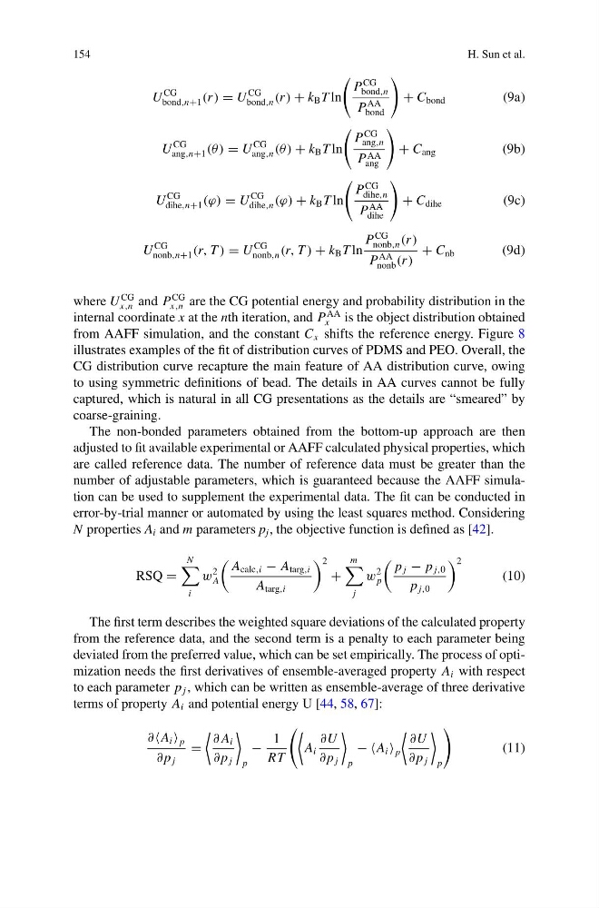
where U
CG
x,n and P
CG
x,n are the CG potential energy and probability distribution in the
internal coordinate x at the nth iteration, and P
AA
x
is the object distribution obtained
from AAFF simulation, and the constant C x shifts the reference energy. Figure 8
illustrates examples of the fit of distribution curves of PDMS and PEO. Overall, the
CG distribution curve recapture the main feature of AA distribution curve, owing
to using symmetric definitions of bead. The details in AA curves cannot be fully
captured, which is natural in all CG presentations as the details are “smeared” by
coarse-graining.
The non-bonded parameters obtained from the bottom-up approach are then
adjusted to fit available experimental or AAFF calculated physical properties, which
are called reference data. The number of reference data must be greater than the
number of adjustable parameters, which is guaranteed because the AAFF simulation can be used to supplement the experimental data. The fit can be conducted in
error-by-trial manner or automated by using the least squares method. Considering
N properties A i and m parameters p j , the objective function is defined as [42].
RSQ =
N
i
w
2
A
A calc,i − A targ,i
A targ,i
2
+
m
j
w
2
p
p j − p j,0
p j,0
2
(10)
The first term describes the weighted square deviations of the calculated property
from the reference data, and the second term is a penalty to each parameter being
deviated from the preferred value, which can be set empirically. The process of optimization needs the first derivatives of ensemble-averaged property A i with respect
to each parameter p j , which can be written as ensemble-average of three derivative
terms of property A i and potential energy U [44, 58, 67]:
∂A i p
∂ p j
=
∂ A i
∂ p j
p
−
1
RT
A i
∂U
∂ p j
p
− A i p
∂U
∂ p j
p
(11)
H. Sun et al.
U
CG
bond,n+1 (r ) = U
CG
bond,n (r ) + k B T ln
P
CG
bond,n
P
AA
bond
+ C bond
(9a)
U
CG
ang,n+1 (θ ) = U
CG
ang,n (θ ) + k B T ln
P
CG
ang,n
P AA
ang
+ C ang
(9b)
U
CG
dihe,n+1 (ϕ) = U
CG
dihe,n (ϕ) + k B T ln
P
CG
dihe,n
P
AA
dihe
+ C dihe
(9c)
U
CG
nonb,n+1 (r, T ) = U
CG
nonb,n (r, T ) + k B T ln
P
CG
nonb,n (r )
P
AA
nonb (r )
+ C nb
(9d)
where U
CG
x,n and P
CG
x,n are the CG potential energy and probability distribution in the
internal coordinate x at the nth iteration, and P
AA
x
is the object distribution obtained
from AAFF simulation, and the constant C x shifts the reference energy. Figure 8
illustrates examples of the fit of distribution curves of PDMS and PEO. Overall, the
CG distribution curve recapture the main feature of AA distribution curve, owing
to using symmetric definitions of bead. The details in AA curves cannot be fully
captured, which is natural in all CG presentations as the details are “smeared” by
coarse-graining.
The non-bonded parameters obtained from the bottom-up approach are then
adjusted to fit available experimental or AAFF calculated physical properties, which
are called reference data. The number of reference data must be greater than the
number of adjustable parameters, which is guaranteed because the AAFF simulation can be used to supplement the experimental data. The fit can be conducted in
error-by-trial manner or automated by using the least squares method. Considering
N properties A i and m parameters p j , the objective function is defined as [42].
RSQ =
N
i
w
2
A
A calc,i − A targ,i
A targ,i
2
+
m
j
w
2
p
p j − p j,0
p j,0
2
(10)
The first term describes the weighted square deviations of the calculated property
from the reference data, and the second term is a penalty to each parameter being
deviated from the preferred value, which can be set empirically. The process of optimization needs the first derivatives of ensemble-averaged property A i with respect
to each parameter p j , which can be written as ensemble-average of three derivative
terms of property A i and potential energy U [44, 58, 67]:
∂A i p
∂ p j
=
∂ A i
∂ p j
p
−
1
RT
A i
∂U
∂ p j
p
− A i p
∂U
∂ p j
p
(11)